 ePub (Kindle)
 Printable PDF
How to measure the accuracy of forecasts

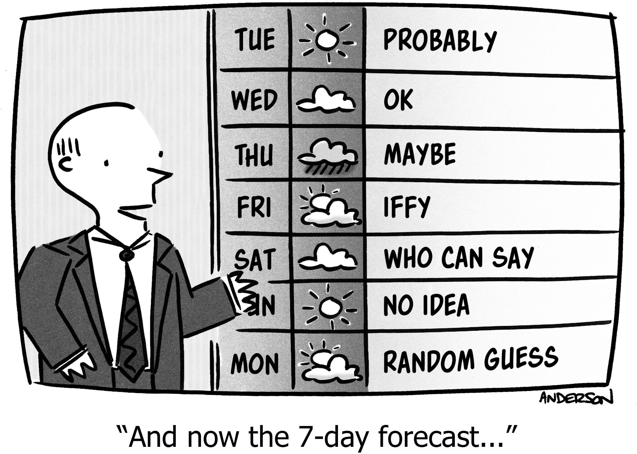
“There’s a 30% chance of rain today.”
And then it didn’t rain. So, was the forecast accurate?
Or it did rain. Is the forecast inaccurate?
How do you hold forecasters accountable, when the forecast is itself a probability? The answer appears tricky, but ends up being simple enough to answer with Google Spreadsheets.
It’s a journey worth taking because of the value of building better forecasts:
- Lead scoring: Putting a value on a new sales lead, predicting the chance of converting to sale, and its dollar value.
- Predicting churn: If you could predict the chance that a given customer will churn in the next thirty days, you could be proactive and perhaps avert the loss; do this enough and you’re on the road to Product/Market Fit.
- Predicting upgrades: If you could predict the chance that a given customer is amenable to an upgrade, you could focus your internal messaging efforts accordingly.
- Risk assessments: Establishing better probabilities on risks results in more intelligent investments.
So how do you measure the accuracy of a prediction that is expressed as a probability? Let’s return to the meteorologist.
Accuracy Error
Clearly, a single data point tells you nothing.
Rather, the correct interpretation of “30% chance of rain” is the following: Gather all the days in which the meteorologist predicted 30%. If the meteorologist is accurate, it will have rained 30% of those times. Similarly, the forecaster will sometimes predict 0% or 10% or 50%. So we should “bucket” the data for each of these predictions, and see what actually happened in each bucket.
What is the right math to determine “how correct” the forecaster is? As is often the answer in statistics, we can take the squared difference1 between the forecast and the actual result.
1 Why do we square the errors instead of using something simpler like the absolute value of the difference? There are two answers. One is that squaring the differences intentionally exaggerates items which are very different from each other. The other is that the mathematics of squared differences is much more tractable than using absolute value. Specifically, you can expand and factor squared differences, and you can use differential calculus. Computing a linear regression line with least-squares, for example, is derived by using calculus to minimize the squared differences, but that same method cannot be applied to linear differences. Nassim Taleb is famously against this practice, but let’s not argue the point now.
Suppose we have two forecasters, and we ask: Who is most accurate? “Accuracy Error” is measured by the sum of the squared differences between the forecast and reality. Whoever has the least total error is the better forecaster.
For example, suppose on some given set of days, forecaster A always predicted a 32% chance of rain, and B always predicted 25%, and suppose in reality it rained on 30% of those days. Then the errors are:
| Predict | Actual | Squared Diff = Error | |
|---|---|---|---|
| A | %22%3E%3Cg%20data-mml-node=%22math%22%3E%3Cg%20data-mml-node=%22mstyle%22%3E%3Cg%20data-mml-node=%22TeXAtom%22%20data-mjx-texclass=%22ORD%22%3E%3Cg%20data-mml-node=%22mn%22%3E%3Cpath%20data-c=%2233%22%20d=%22M127%20463q-27%200-42%2017T69%20524q0%2055%2048%2098t116%2043q35%200%2044-1%2074-12%20113-53t40-89q0-52-34-101t-94-71l-3-2q0-1%209-3t29-9%2038-21q82-53%2082-140%200-79-62-138T238-22q-80%200-138%2043T42%20130q0%2028%2018%2045t45%2018q28%200%2046-18t18-45q0-11-3-20t-7-16-11-12-12-8-10-4-8-3l-4-1q51-45%20124-45%2055%200%2083%2053%2017%2033%2017%20101v20q0%2095-64%20127-15%206-61%207l-42%201-3%202q-2%203-2%2016%200%2018%208%2018%2028%200%2058%205%2034%205%2062%2042t28%20112v8q0%2057-35%2079-22%2014-47%2014-32%200-59-11t-38-23-11-12h3q3-1%208-2t10-5%2012-7%2010-11%208-15%203-20q0-22-14-39t-45-18z%22/%3E%3Cpath%20data-c=%2232%22%20d=%22M109%20429q-27%200-43%2018T50%20491q0%2071%2053%20123t132%2052q91%200%20152-56t62-145q0-43-20-82t-48-68-80-74q-36-31-1e2-92L142%2093l76-1q157%200%20167%205%207%202%2024%2089v3h40v-3q-1-3-13-91T421%203V0H50V19%2031q0%207%206%2015T86%2081q29%2032%2050%2056%209%2010%2034%2037t34%2037%2029%2033%2028%2034%2023%2030%2021%2032%2015%2029%2013%2032%207%2030%203%2033q0%2063-34%20109t-97%2046q-33%200-58-17t-35-33-10-19q0-1%205-1%2018%200%2037-14t19-46q0-25-16-42t-45-18z%22%20transform=%22translate(500,0)%22/%3E%3C/g%3E%3Cg%20data-mml-node=%22mi%22%20transform=%22translate(1000,0)%22%3E%3Cpath%20data-c=%2225%22%20d=%22M465%20605q-37%200-71%209t-54%2018-21%209q13-33%2013-93%200-90-39-145t-91-56q-57%200-101%2055T56%20548q0%2089%2045%20145t101%2057q39%200%2070-31%2087-77%20192-77%20116%200%20186%2090%2012%2016%2018%2017%202%201%205%201%209%200%2015-7t5-17Q178-47%20170-52q-4-4-10-4-13%200-18%2011-5%209%200%2018%201%203%20221%20331Q469%20462%20525%20546l56%2084q-53-25-116-25zM207%20385q28%200%2056%2042t29%20121q0%2069-25%20116t-67%2048q-7%200-14-3t-19-11-20-30-13-53q-2-20-2-67V527q0-91%2033-124%2018-18%2038-18h4zM5e2%20146q0%2088%2044%20144t103%2057q52%200%2090-55t39-146T737%200%20646-56Q590-56%20545%200T5e2%20146zM651-18q28%200%2056%2042t29%20122q0%2069-25%20116t-67%2047q-7%200-14-3t-19-11-20-30-13-53q-1-12-1-66V124q0-142%2070-142h4z%22/%3E%3C/g%3E%3C/g%3E%3C/g%3E%3C/g%3E%3C/g%3E%3C/svg%3E) |
%22%3E%3Cg%20data-mml-node=%22math%22%3E%3Cg%20data-mml-node=%22mstyle%22%3E%3Cg%20data-mml-node=%22TeXAtom%22%20data-mjx-texclass=%22ORD%22%3E%3Cg%20data-mml-node=%22mn%22%3E%3Cpath%20data-c=%2233%22%20d=%22M127%20463q-27%200-42%2017T69%20524q0%2055%2048%2098t116%2043q35%200%2044-1%2074-12%20113-53t40-89q0-52-34-101t-94-71l-3-2q0-1%209-3t29-9%2038-21q82-53%2082-140%200-79-62-138T238-22q-80%200-138%2043T42%20130q0%2028%2018%2045t45%2018q28%200%2046-18t18-45q0-11-3-20t-7-16-11-12-12-8-10-4-8-3l-4-1q51-45%20124-45%2055%200%2083%2053%2017%2033%2017%20101v20q0%2095-64%20127-15%206-61%207l-42%201-3%202q-2%203-2%2016%200%2018%208%2018%2028%200%2058%205%2034%205%2062%2042t28%20112v8q0%2057-35%2079-22%2014-47%2014-32%200-59-11t-38-23-11-12h3q3-1%208-2t10-5%2012-7%2010-11%208-15%203-20q0-22-14-39t-45-18z%22/%3E%3Cpath%20data-c=%2230%22%20d=%22M96%20585q56%2081%20153%2081%2048%200%2096-26t78-92q37-83%2037-228%200-155-43-237-20-42-55-67T301-15t-51-7q-26%200-52%206T137%2016%2082%2083Q39%20165%2039%20320q0%20174%2057%20265zm225%2012q-30%2032-71%2032-42%200-72-32-25-26-33-72t-8-192q0-158%208-208t36-79q28-30%2069-30%2040%200%2068%2030%2029%2030%2036%2084t8%20203q0%20145-8%20191t-33%2073z%22%20transform=%22translate(500,0)%22/%3E%3C/g%3E%3Cg%20data-mml-node=%22mi%22%20transform=%22translate(1000,0)%22%3E%3Cpath%20data-c=%2225%22%20d=%22M465%20605q-37%200-71%209t-54%2018-21%209q13-33%2013-93%200-90-39-145t-91-56q-57%200-101%2055T56%20548q0%2089%2045%20145t101%2057q39%200%2070-31%2087-77%20192-77%20116%200%20186%2090%2012%2016%2018%2017%202%201%205%201%209%200%2015-7t5-17Q178-47%20170-52q-4-4-10-4-13%200-18%2011-5%209%200%2018%201%203%20221%20331Q469%20462%20525%20546l56%2084q-53-25-116-25zM207%20385q28%200%2056%2042t29%20121q0%2069-25%20116t-67%2048q-7%200-14-3t-19-11-20-30-13-53q-2-20-2-67V527q0-91%2033-124%2018-18%2038-18h4zM5e2%20146q0%2088%2044%20144t103%2057q52%200%2090-55t39-146T737%200%20646-56Q590-56%20545%200T5e2%20146zM651-18q28%200%2056%2042t29%20122q0%2069-25%20116t-67%2047q-7%200-14-3t-19-11-20-30-13-53q-1-12-1-66V124q0-142%2070-142h4z%22/%3E%3C/g%3E%3C/g%3E%3C/g%3E%3C/g%3E%3C/g%3E%3C/svg%3E) |
%22%3E%3Cg%20data-mml-node=%22math%22%3E%3Cg%20data-mml-node=%22mstyle%22%3E%3Cg%20data-mml-node=%22TeXAtom%22%20data-mjx-texclass=%22ORD%22%3E%3Cg%20data-mml-node=%22mo%22%3E%3Cpath%20data-c=%2228%22%20d=%22M94%20250q0%2069%2010%20131t23%20107%2037%2088%2038%2067%2042%2052%2033%2034%2025%2021h13%204q14%200%2014-9%200-3-17-21t-41-53-49-86-42-138-17-193T184%2058%20225-81t49-86%2042-53%2017-21q0-9-15-9h-3-13l-28%2024Q180-141%20137-14T94%20250z%22/%3E%3C/g%3E%3Cg%20data-mml-node=%22mn%22%20transform=%22translate(389,0)%22%3E%3Cpath%20data-c=%2230%22%20d=%22M96%20585q56%2081%20153%2081%2048%200%2096-26t78-92q37-83%2037-228%200-155-43-237-20-42-55-67T301-15t-51-7q-26%200-52%206T137%2016%2082%2083Q39%20165%2039%20320q0%20174%2057%20265zm225%2012q-30%2032-71%2032-42%200-72-32-25-26-33-72t-8-192q0-158%208-208t36-79q28-30%2069-30%2040%200%2068%2030%2029%2030%2036%2084t8%20203q0%20145-8%20191t-33%2073z%22/%3E%3Cpath%20data-c=%222E%22%20d=%22M78%2060q0%2024%2017%2042t43%2018q24%200%2042-16t19-43q0-25-17-43T139%200%2096%2017%2078%2060z%22%20transform=%22translate(500,0)%22/%3E%3Cpath%20data-c=%2233%22%20d=%22M127%20463q-27%200-42%2017T69%20524q0%2055%2048%2098t116%2043q35%200%2044-1%2074-12%20113-53t40-89q0-52-34-101t-94-71l-3-2q0-1%209-3t29-9%2038-21q82-53%2082-140%200-79-62-138T238-22q-80%200-138%2043T42%20130q0%2028%2018%2045t45%2018q28%200%2046-18t18-45q0-11-3-20t-7-16-11-12-12-8-10-4-8-3l-4-1q51-45%20124-45%2055%200%2083%2053%2017%2033%2017%20101v20q0%2095-64%20127-15%206-61%207l-42%201-3%202q-2%203-2%2016%200%2018%208%2018%2028%200%2058%205%2034%205%2062%2042t28%20112v8q0%2057-35%2079-22%2014-47%2014-32%200-59-11t-38-23-11-12h3q3-1%208-2t10-5%2012-7%2010-11%208-15%203-20q0-22-14-39t-45-18z%22%20transform=%22translate(778,0)%22/%3E%3Cpath%20data-c=%2232%22%20d=%22M109%20429q-27%200-43%2018T50%20491q0%2071%2053%20123t132%2052q91%200%20152-56t62-145q0-43-20-82t-48-68-80-74q-36-31-1e2-92L142%2093l76-1q157%200%20167%205%207%202%2024%2089v3h40v-3q-1-3-13-91T421%203V0H50V19%2031q0%207%206%2015T86%2081q29%2032%2050%2056%209%2010%2034%2037t34%2037%2029%2033%2028%2034%2023%2030%2021%2032%2015%2029%2013%2032%207%2030%203%2033q0%2063-34%20109t-97%2046q-33%200-58-17t-35-33-10-19q0-1%205-1%2018%200%2037-14t19-46q0-25-16-42t-45-18z%22%20transform=%22translate(1278,0)%22/%3E%3C/g%3E%3Cg%20data-mml-node=%22mo%22%20transform=%22translate(2389.2,0)%22%3E%3Cpath%20data-c=%222212%22%20d=%22M84%20237t0%2013%2014%2020H679q15-8%2015-20t-15-20H98q-14%207-14%2020z%22/%3E%3C/g%3E%3Cg%20data-mml-node=%22mn%22%20transform=%22translate(3389.4,0)%22%3E%3Cpath%20data-c=%2230%22%20d=%22M96%20585q56%2081%20153%2081%2048%200%2096-26t78-92q37-83%2037-228%200-155-43-237-20-42-55-67T301-15t-51-7q-26%200-52%206T137%2016%2082%2083Q39%20165%2039%20320q0%20174%2057%20265zm225%2012q-30%2032-71%2032-42%200-72-32-25-26-33-72t-8-192q0-158%208-208t36-79q28-30%2069-30%2040%200%2068%2030%2029%2030%2036%2084t8%20203q0%20145-8%20191t-33%2073z%22/%3E%3Cpath%20data-c=%222E%22%20d=%22M78%2060q0%2024%2017%2042t43%2018q24%200%2042-16t19-43q0-25-17-43T139%200%2096%2017%2078%2060z%22%20transform=%22translate(500,0)%22/%3E%3Cpath%20data-c=%2233%22%20d=%22M127%20463q-27%200-42%2017T69%20524q0%2055%2048%2098t116%2043q35%200%2044-1%2074-12%20113-53t40-89q0-52-34-101t-94-71l-3-2q0-1%209-3t29-9%2038-21q82-53%2082-140%200-79-62-138T238-22q-80%200-138%2043T42%20130q0%2028%2018%2045t45%2018q28%200%2046-18t18-45q0-11-3-20t-7-16-11-12-12-8-10-4-8-3l-4-1q51-45%20124-45%2055%200%2083%2053%2017%2033%2017%20101v20q0%2095-64%20127-15%206-61%207l-42%201-3%202q-2%203-2%2016%200%2018%208%2018%2028%200%2058%205%2034%205%2062%2042t28%20112v8q0%2057-35%2079-22%2014-47%2014-32%200-59-11t-38-23-11-12h3q3-1%208-2t10-5%2012-7%2010-11%208-15%203-20q0-22-14-39t-45-18z%22%20transform=%22translate(778,0)%22/%3E%3Cpath%20data-c=%2230%22%20d=%22M96%20585q56%2081%20153%2081%2048%200%2096-26t78-92q37-83%2037-228%200-155-43-237-20-42-55-67T301-15t-51-7q-26%200-52%206T137%2016%2082%2083Q39%20165%2039%20320q0%20174%2057%20265zm225%2012q-30%2032-71%2032-42%200-72-32-25-26-33-72t-8-192q0-158%208-208t36-79q28-30%2069-30%2040%200%2068%2030%2029%2030%2036%2084t8%20203q0%20145-8%20191t-33%2073z%22%20transform=%22translate(1278,0)%22/%3E%3C/g%3E%3Cg%20data-mml-node=%22msup%22%20transform=%22translate(5167.4,0)%22%3E%3Cg%20data-mml-node=%22mo%22%3E%3Cpath%20data-c=%2229%22%20d=%22M60%20749l4%201q5%200%2010%200H86l28-24q94-85%20137-212t43-264q0-68-10-131T261%2012%20224-76t-38-67-41-51-32-33-23-19q-3-3-4-4H74q-8%200-11%200t-5%203-3%209q1%201%2011%2013Q221-64%20221%20250T66%20725q-10%2012-11%2013%200%208%205%2011z%22/%3E%3C/g%3E%3Cg%20data-mml-node=%22mn%22%20transform=%22translate(422,363)%20scale(0.707)%22%3E%3Cpath%20data-c=%2232%22%20d=%22M109%20429q-27%200-43%2018T50%20491q0%2071%2053%20123t132%2052q91%200%20152-56t62-145q0-43-20-82t-48-68-80-74q-36-31-1e2-92L142%2093l76-1q157%200%20167%205%207%202%2024%2089v3h40v-3q-1-3-13-91T421%203V0H50V19%2031q0%207%206%2015T86%2081q29%2032%2050%2056%209%2010%2034%2037t34%2037%2029%2033%2028%2034%2023%2030%2021%2032%2015%2029%2013%2032%207%2030%203%2033q0%2063-34%20109t-97%2046q-33%200-58-17t-35-33-10-19q0-1%205-1%2018%200%2037-14t19-46q0-25-16-42t-45-18z%22/%3E%3C/g%3E%3C/g%3E%3Cg%20data-mml-node=%22mo%22%20transform=%22translate(6270.8,0)%22%3E%3Cpath%20data-c=%223D%22%20d=%22M56%20347q0%2013%2014%2020H707q15-8%2015-20%200-11-14-19l-318-1H72q-16%205-16%2020zm0-194q0%2015%2016%2020H708q14-10%2014-20%200-13-15-20H70q-14%207-14%2020z%22/%3E%3C/g%3E%3Cg%20data-mml-node=%22mn%22%20transform=%22translate(7326.6,0)%22%3E%3Cpath%20data-c=%2230%22%20d=%22M96%20585q56%2081%20153%2081%2048%200%2096-26t78-92q37-83%2037-228%200-155-43-237-20-42-55-67T301-15t-51-7q-26%200-52%206T137%2016%2082%2083Q39%20165%2039%20320q0%20174%2057%20265zm225%2012q-30%2032-71%2032-42%200-72-32-25-26-33-72t-8-192q0-158%208-208t36-79q28-30%2069-30%2040%200%2068%2030%2029%2030%2036%2084t8%20203q0%20145-8%20191t-33%2073z%22/%3E%3Cpath%20data-c=%222E%22%20d=%22M78%2060q0%2024%2017%2042t43%2018q24%200%2042-16t19-43q0-25-17-43T139%200%2096%2017%2078%2060z%22%20transform=%22translate(500,0)%22/%3E%3Cpath%20data-c=%2230%22%20d=%22M96%20585q56%2081%20153%2081%2048%200%2096-26t78-92q37-83%2037-228%200-155-43-237-20-42-55-67T301-15t-51-7q-26%200-52%206T137%2016%2082%2083Q39%20165%2039%20320q0%20174%2057%20265zm225%2012q-30%2032-71%2032-42%200-72-32-25-26-33-72t-8-192q0-158%208-208t36-79q28-30%2069-30%2040%200%2068%2030%2029%2030%2036%2084t8%20203q0%20145-8%20191t-33%2073z%22%20transform=%22translate(778,0)%22/%3E%3Cpath%20data-c=%2230%22%20d=%22M96%20585q56%2081%20153%2081%2048%200%2096-26t78-92q37-83%2037-228%200-155-43-237-20-42-55-67T301-15t-51-7q-26%200-52%206T137%2016%2082%2083Q39%20165%2039%20320q0%20174%2057%20265zm225%2012q-30%2032-71%2032-42%200-72-32-25-26-33-72t-8-192q0-158%208-208t36-79q28-30%2069-30%2040%200%2068%2030%2029%2030%2036%2084t8%20203q0%20145-8%20191t-33%2073z%22%20transform=%22translate(1278,0)%22/%3E%3Cpath%20data-c=%2230%22%20d=%22M96%20585q56%2081%20153%2081%2048%200%2096-26t78-92q37-83%2037-228%200-155-43-237-20-42-55-67T301-15t-51-7q-26%200-52%206T137%2016%2082%2083Q39%20165%2039%20320q0%20174%2057%20265zm225%2012q-30%2032-71%2032-42%200-72-32-25-26-33-72t-8-192q0-158%208-208t36-79q28-30%2069-30%2040%200%2068%2030%2029%2030%2036%2084t8%20203q0%20145-8%20191t-33%2073z%22%20transform=%22translate(1778,0)%22/%3E%3Cpath%20data-c=%2234%22%20d=%22M462%200Q444%203%20333%203%20217%203%20199%200h-9V46h31q20%200%2027%200t17%202%2014%205%207%208q1%202%201%2054v50H28v46L179%20442Q332%20674%20334%20675q2%202%2021%202h18l6-6V211h92V165H379V114q0-41%200-48t6-12q8-7%2057-8h29V0h-9zM293%20211V545L74%20212l109-1H293z%22%20transform=%22translate(2278,0)%22/%3E%3C/g%3E%3C/g%3E%3C/g%3E%3C/g%3E%3C/g%3E%3C/svg%3E) |
| B | %22%3E%3Cg%20data-mml-node=%22math%22%3E%3Cg%20data-mml-node=%22mstyle%22%3E%3Cg%20data-mml-node=%22TeXAtom%22%20data-mjx-texclass=%22ORD%22%3E%3Cg%20data-mml-node=%22mn%22%3E%3Cpath%20data-c=%2232%22%20d=%22M109%20429q-27%200-43%2018T50%20491q0%2071%2053%20123t132%2052q91%200%20152-56t62-145q0-43-20-82t-48-68-80-74q-36-31-1e2-92L142%2093l76-1q157%200%20167%205%207%202%2024%2089v3h40v-3q-1-3-13-91T421%203V0H50V19%2031q0%207%206%2015T86%2081q29%2032%2050%2056%209%2010%2034%2037t34%2037%2029%2033%2028%2034%2023%2030%2021%2032%2015%2029%2013%2032%207%2030%203%2033q0%2063-34%20109t-97%2046q-33%200-58-17t-35-33-10-19q0-1%205-1%2018%200%2037-14t19-46q0-25-16-42t-45-18z%22/%3E%3Cpath%20data-c=%2235%22%20d=%22M164%20157q0-24-16-40t-39-16h-7q46-79%20122-79%2070%200%20102%2060%2019%2033%2019%20128%200%20103-27%20139-26%2033-58%2033h-6q-78%200-118-68-4-7-7-8t-15-2q-17%200-19%206-2%204-2%20175V614q0%2050%205%2050%202%202%204%202%201%200%2021-8t55-16%2075-8q71%200%20136%2028%208%204%2013%204%208%200%208-18V635q-82-97-205-97-31%200-56%206l-10%202V374q19%2014%2030%2022t36%2016%2051%208q81%200%20137-65t56-154q0-92-64-157T229-22Q148-22%2099%2032T50%20154q0%2024%2011%2038t23%2018%2023%204q25%200%2041-17t16-40z%22%20transform=%22translate(500,0)%22/%3E%3C/g%3E%3Cg%20data-mml-node=%22mi%22%20transform=%22translate(1000,0)%22%3E%3Cpath%20data-c=%2225%22%20d=%22M465%20605q-37%200-71%209t-54%2018-21%209q13-33%2013-93%200-90-39-145t-91-56q-57%200-101%2055T56%20548q0%2089%2045%20145t101%2057q39%200%2070-31%2087-77%20192-77%20116%200%20186%2090%2012%2016%2018%2017%202%201%205%201%209%200%2015-7t5-17Q178-47%20170-52q-4-4-10-4-13%200-18%2011-5%209%200%2018%201%203%20221%20331Q469%20462%20525%20546l56%2084q-53-25-116-25zM207%20385q28%200%2056%2042t29%20121q0%2069-25%20116t-67%2048q-7%200-14-3t-19-11-20-30-13-53q-2-20-2-67V527q0-91%2033-124%2018-18%2038-18h4zM5e2%20146q0%2088%2044%20144t103%2057q52%200%2090-55t39-146T737%200%20646-56Q590-56%20545%200T5e2%20146zM651-18q28%200%2056%2042t29%20122q0%2069-25%20116t-67%2047q-7%200-14-3t-19-11-20-30-13-53q-1-12-1-66V124q0-142%2070-142h4z%22/%3E%3C/g%3E%3C/g%3E%3C/g%3E%3C/g%3E%3C/g%3E%3C/svg%3E) |
|
%22%3E%3Cg%20data-mml-node=%22math%22%3E%3Cg%20data-mml-node=%22mstyle%22%3E%3Cg%20data-mml-node=%22TeXAtom%22%20data-mjx-texclass=%22ORD%22%3E%3Cg%20data-mml-node=%22mo%22%3E%3Cpath%20data-c=%2228%22%20d=%22M94%20250q0%2069%2010%20131t23%20107%2037%2088%2038%2067%2042%2052%2033%2034%2025%2021h13%204q14%200%2014-9%200-3-17-21t-41-53-49-86-42-138-17-193T184%2058%20225-81t49-86%2042-53%2017-21q0-9-15-9h-3-13l-28%2024Q180-141%20137-14T94%20250z%22/%3E%3C/g%3E%3Cg%20data-mml-node=%22mn%22%20transform=%22translate(389,0)%22%3E%3Cpath%20data-c=%2230%22%20d=%22M96%20585q56%2081%20153%2081%2048%200%2096-26t78-92q37-83%2037-228%200-155-43-237-20-42-55-67T301-15t-51-7q-26%200-52%206T137%2016%2082%2083Q39%20165%2039%20320q0%20174%2057%20265zm225%2012q-30%2032-71%2032-42%200-72-32-25-26-33-72t-8-192q0-158%208-208t36-79q28-30%2069-30%2040%200%2068%2030%2029%2030%2036%2084t8%20203q0%20145-8%20191t-33%2073z%22/%3E%3Cpath%20data-c=%222E%22%20d=%22M78%2060q0%2024%2017%2042t43%2018q24%200%2042-16t19-43q0-25-17-43T139%200%2096%2017%2078%2060z%22%20transform=%22translate(500,0)%22/%3E%3Cpath%20data-c=%2232%22%20d=%22M109%20429q-27%200-43%2018T50%20491q0%2071%2053%20123t132%2052q91%200%20152-56t62-145q0-43-20-82t-48-68-80-74q-36-31-1e2-92L142%2093l76-1q157%200%20167%205%207%202%2024%2089v3h40v-3q-1-3-13-91T421%203V0H50V19%2031q0%207%206%2015T86%2081q29%2032%2050%2056%209%2010%2034%2037t34%2037%2029%2033%2028%2034%2023%2030%2021%2032%2015%2029%2013%2032%207%2030%203%2033q0%2063-34%20109t-97%2046q-33%200-58-17t-35-33-10-19q0-1%205-1%2018%200%2037-14t19-46q0-25-16-42t-45-18z%22%20transform=%22translate(778,0)%22/%3E%3Cpath%20data-c=%2235%22%20d=%22M164%20157q0-24-16-40t-39-16h-7q46-79%20122-79%2070%200%20102%2060%2019%2033%2019%20128%200%20103-27%20139-26%2033-58%2033h-6q-78%200-118-68-4-7-7-8t-15-2q-17%200-19%206-2%204-2%20175V614q0%2050%205%2050%202%202%204%202%201%200%2021-8t55-16%2075-8q71%200%20136%2028%208%204%2013%204%208%200%208-18V635q-82-97-205-97-31%200-56%206l-10%202V374q19%2014%2030%2022t36%2016%2051%208q81%200%20137-65t56-154q0-92-64-157T229-22Q148-22%2099%2032T50%20154q0%2024%2011%2038t23%2018%2023%204q25%200%2041-17t16-40z%22%20transform=%22translate(1278,0)%22/%3E%3C/g%3E%3Cg%20data-mml-node=%22mo%22%20transform=%22translate(2389.2,0)%22%3E%3Cpath%20data-c=%222212%22%20d=%22M84%20237t0%2013%2014%2020H679q15-8%2015-20t-15-20H98q-14%207-14%2020z%22/%3E%3C/g%3E%3Cg%20data-mml-node=%22mn%22%20transform=%22translate(3389.4,0)%22%3E%3Cpath%20data-c=%2230%22%20d=%22M96%20585q56%2081%20153%2081%2048%200%2096-26t78-92q37-83%2037-228%200-155-43-237-20-42-55-67T301-15t-51-7q-26%200-52%206T137%2016%2082%2083Q39%20165%2039%20320q0%20174%2057%20265zm225%2012q-30%2032-71%2032-42%200-72-32-25-26-33-72t-8-192q0-158%208-208t36-79q28-30%2069-30%2040%200%2068%2030%2029%2030%2036%2084t8%20203q0%20145-8%20191t-33%2073z%22/%3E%3Cpath%20data-c=%222E%22%20d=%22M78%2060q0%2024%2017%2042t43%2018q24%200%2042-16t19-43q0-25-17-43T139%200%2096%2017%2078%2060z%22%20transform=%22translate(500,0)%22/%3E%3Cpath%20data-c=%2233%22%20d=%22M127%20463q-27%200-42%2017T69%20524q0%2055%2048%2098t116%2043q35%200%2044-1%2074-12%20113-53t40-89q0-52-34-101t-94-71l-3-2q0-1%209-3t29-9%2038-21q82-53%2082-140%200-79-62-138T238-22q-80%200-138%2043T42%20130q0%2028%2018%2045t45%2018q28%200%2046-18t18-45q0-11-3-20t-7-16-11-12-12-8-10-4-8-3l-4-1q51-45%20124-45%2055%200%2083%2053%2017%2033%2017%20101v20q0%2095-64%20127-15%206-61%207l-42%201-3%202q-2%203-2%2016%200%2018%208%2018%2028%200%2058%205%2034%205%2062%2042t28%20112v8q0%2057-35%2079-22%2014-47%2014-32%200-59-11t-38-23-11-12h3q3-1%208-2t10-5%2012-7%2010-11%208-15%203-20q0-22-14-39t-45-18z%22%20transform=%22translate(778,0)%22/%3E%3Cpath%20data-c=%2230%22%20d=%22M96%20585q56%2081%20153%2081%2048%200%2096-26t78-92q37-83%2037-228%200-155-43-237-20-42-55-67T301-15t-51-7q-26%200-52%206T137%2016%2082%2083Q39%20165%2039%20320q0%20174%2057%20265zm225%2012q-30%2032-71%2032-42%200-72-32-25-26-33-72t-8-192q0-158%208-208t36-79q28-30%2069-30%2040%200%2068%2030%2029%2030%2036%2084t8%20203q0%20145-8%20191t-33%2073z%22%20transform=%22translate(1278,0)%22/%3E%3C/g%3E%3Cg%20data-mml-node=%22msup%22%20transform=%22translate(5167.4,0)%22%3E%3Cg%20data-mml-node=%22mo%22%3E%3Cpath%20data-c=%2229%22%20d=%22M60%20749l4%201q5%200%2010%200H86l28-24q94-85%20137-212t43-264q0-68-10-131T261%2012%20224-76t-38-67-41-51-32-33-23-19q-3-3-4-4H74q-8%200-11%200t-5%203-3%209q1%201%2011%2013Q221-64%20221%20250T66%20725q-10%2012-11%2013%200%208%205%2011z%22/%3E%3C/g%3E%3Cg%20data-mml-node=%22mn%22%20transform=%22translate(422,363)%20scale(0.707)%22%3E%3Cpath%20data-c=%2232%22%20d=%22M109%20429q-27%200-43%2018T50%20491q0%2071%2053%20123t132%2052q91%200%20152-56t62-145q0-43-20-82t-48-68-80-74q-36-31-1e2-92L142%2093l76-1q157%200%20167%205%207%202%2024%2089v3h40v-3q-1-3-13-91T421%203V0H50V19%2031q0%207%206%2015T86%2081q29%2032%2050%2056%209%2010%2034%2037t34%2037%2029%2033%2028%2034%2023%2030%2021%2032%2015%2029%2013%2032%207%2030%203%2033q0%2063-34%20109t-97%2046q-33%200-58-17t-35-33-10-19q0-1%205-1%2018%200%2037-14t19-46q0-25-16-42t-45-18z%22/%3E%3C/g%3E%3C/g%3E%3Cg%20data-mml-node=%22mo%22%20transform=%22translate(6270.8,0)%22%3E%3Cpath%20data-c=%223D%22%20d=%22M56%20347q0%2013%2014%2020H707q15-8%2015-20%200-11-14-19l-318-1H72q-16%205-16%2020zm0-194q0%2015%2016%2020H708q14-10%2014-20%200-13-15-20H70q-14%207-14%2020z%22/%3E%3C/g%3E%3Cg%20data-mml-node=%22mn%22%20transform=%22translate(7326.6,0)%22%3E%3Cpath%20data-c=%2230%22%20d=%22M96%20585q56%2081%20153%2081%2048%200%2096-26t78-92q37-83%2037-228%200-155-43-237-20-42-55-67T301-15t-51-7q-26%200-52%206T137%2016%2082%2083Q39%20165%2039%20320q0%20174%2057%20265zm225%2012q-30%2032-71%2032-42%200-72-32-25-26-33-72t-8-192q0-158%208-208t36-79q28-30%2069-30%2040%200%2068%2030%2029%2030%2036%2084t8%20203q0%20145-8%20191t-33%2073z%22/%3E%3Cpath%20data-c=%222E%22%20d=%22M78%2060q0%2024%2017%2042t43%2018q24%200%2042-16t19-43q0-25-17-43T139%200%2096%2017%2078%2060z%22%20transform=%22translate(500,0)%22/%3E%3Cpath%20data-c=%2230%22%20d=%22M96%20585q56%2081%20153%2081%2048%200%2096-26t78-92q37-83%2037-228%200-155-43-237-20-42-55-67T301-15t-51-7q-26%200-52%206T137%2016%2082%2083Q39%20165%2039%20320q0%20174%2057%20265zm225%2012q-30%2032-71%2032-42%200-72-32-25-26-33-72t-8-192q0-158%208-208t36-79q28-30%2069-30%2040%200%2068%2030%2029%2030%2036%2084t8%20203q0%20145-8%20191t-33%2073z%22%20transform=%22translate(778,0)%22/%3E%3Cpath%20data-c=%2230%22%20d=%22M96%20585q56%2081%20153%2081%2048%200%2096-26t78-92q37-83%2037-228%200-155-43-237-20-42-55-67T301-15t-51-7q-26%200-52%206T137%2016%2082%2083Q39%20165%2039%20320q0%20174%2057%20265zm225%2012q-30%2032-71%2032-42%200-72-32-25-26-33-72t-8-192q0-158%208-208t36-79q28-30%2069-30%2040%200%2068%2030%2029%2030%2036%2084t8%20203q0%20145-8%20191t-33%2073z%22%20transform=%22translate(1278,0)%22/%3E%3Cpath%20data-c=%2232%22%20d=%22M109%20429q-27%200-43%2018T50%20491q0%2071%2053%20123t132%2052q91%200%20152-56t62-145q0-43-20-82t-48-68-80-74q-36-31-1e2-92L142%2093l76-1q157%200%20167%205%207%202%2024%2089v3h40v-3q-1-3-13-91T421%203V0H50V19%2031q0%207%206%2015T86%2081q29%2032%2050%2056%209%2010%2034%2037t34%2037%2029%2033%2028%2034%2023%2030%2021%2032%2015%2029%2013%2032%207%2030%203%2033q0%2063-34%20109t-97%2046q-33%200-58-17t-35-33-10-19q0-1%205-1%2018%200%2037-14t19-46q0-25-16-42t-45-18z%22%20transform=%22translate(1778,0)%22/%3E%3Cpath%20data-c=%2235%22%20d=%22M164%20157q0-24-16-40t-39-16h-7q46-79%20122-79%2070%200%20102%2060%2019%2033%2019%20128%200%20103-27%20139-26%2033-58%2033h-6q-78%200-118-68-4-7-7-8t-15-2q-17%200-19%206-2%204-2%20175V614q0%2050%205%2050%202%202%204%202%201%200%2021-8t55-16%2075-8q71%200%20136%2028%208%204%2013%204%208%200%208-18V635q-82-97-205-97-31%200-56%206l-10%202V374q19%2014%2030%2022t36%2016%2051%208q81%200%20137-65t56-154q0-92-64-157T229-22Q148-22%2099%2032T50%20154q0%2024%2011%2038t23%2018%2023%204q25%200%2041-17t16-40z%22%20transform=%22translate(2278,0)%22/%3E%3C/g%3E%3C/g%3E%3C/g%3E%3C/g%3E%3C/g%3E%3C/svg%3E) |
It feels like we’re finished, but alas no. If all we compute is Accuracy Error, we fall for a trap in which we easily forecast with perfect accuracy, while also being utterly useless.
Discernment
Suppose these meteorologists are in a region that rains 110 days out of every 365. That is, the overall climactic average probability of rain is 30%. A meteorologist would know that. So, a meteorologist could simply predict “30% chance of rain” every single day, no matter what. Easy job!
Our Accuracy Error metric will report that this forecaster is perfect—exactly zero over a whole year of predictions. Because, the prediction is always 30%, and indeed on those days it rained 30% of the time: %22%3E%3Cg%20data-mml-node=%22math%22%3E%3Cg%20data-mml-node=%22mstyle%22%3E%3Cg%20data-mml-node=%22TeXAtom%22%20data-mjx-texclass=%22ORD%22%3E%3Cg%20data-mml-node=%22mo%22%3E%3Cpath%20data-c=%2228%22%20d=%22M94%20250q0%2069%2010%20131t23%20107%2037%2088%2038%2067%2042%2052%2033%2034%2025%2021h13%204q14%200%2014-9%200-3-17-21t-41-53-49-86-42-138-17-193T184%2058%20225-81t49-86%2042-53%2017-21q0-9-15-9h-3-13l-28%2024Q180-141%20137-14T94%20250z%22/%3E%3C/g%3E%3Cg%20data-mml-node=%22mn%22%20transform=%22translate(389,0)%22%3E%3Cpath%20data-c=%2230%22%20d=%22M96%20585q56%2081%20153%2081%2048%200%2096-26t78-92q37-83%2037-228%200-155-43-237-20-42-55-67T301-15t-51-7q-26%200-52%206T137%2016%2082%2083Q39%20165%2039%20320q0%20174%2057%20265zm225%2012q-30%2032-71%2032-42%200-72-32-25-26-33-72t-8-192q0-158%208-208t36-79q28-30%2069-30%2040%200%2068%2030%2029%2030%2036%2084t8%20203q0%20145-8%20191t-33%2073z%22/%3E%3Cpath%20data-c=%222E%22%20d=%22M78%2060q0%2024%2017%2042t43%2018q24%200%2042-16t19-43q0-25-17-43T139%200%2096%2017%2078%2060z%22%20transform=%22translate(500,0)%22/%3E%3Cpath%20data-c=%2233%22%20d=%22M127%20463q-27%200-42%2017T69%20524q0%2055%2048%2098t116%2043q35%200%2044-1%2074-12%20113-53t40-89q0-52-34-101t-94-71l-3-2q0-1%209-3t29-9%2038-21q82-53%2082-140%200-79-62-138T238-22q-80%200-138%2043T42%20130q0%2028%2018%2045t45%2018q28%200%2046-18t18-45q0-11-3-20t-7-16-11-12-12-8-10-4-8-3l-4-1q51-45%20124-45%2055%200%2083%2053%2017%2033%2017%20101v20q0%2095-64%20127-15%206-61%207l-42%201-3%202q-2%203-2%2016%200%2018%208%2018%2028%200%2058%205%2034%205%2062%2042t28%20112v8q0%2057-35%2079-22%2014-47%2014-32%200-59-11t-38-23-11-12h3q3-1%208-2t10-5%2012-7%2010-11%208-15%203-20q0-22-14-39t-45-18z%22%20transform=%22translate(778,0)%22/%3E%3Cpath%20data-c=%2230%22%20d=%22M96%20585q56%2081%20153%2081%2048%200%2096-26t78-92q37-83%2037-228%200-155-43-237-20-42-55-67T301-15t-51-7q-26%200-52%206T137%2016%2082%2083Q39%20165%2039%20320q0%20174%2057%20265zm225%2012q-30%2032-71%2032-42%200-72-32-25-26-33-72t-8-192q0-158%208-208t36-79q28-30%2069-30%2040%200%2068%2030%2029%2030%2036%2084t8%20203q0%20145-8%20191t-33%2073z%22%20transform=%22translate(1278,0)%22/%3E%3C/g%3E%3Cg%20data-mml-node=%22mo%22%20transform=%22translate(2389.2,0)%22%3E%3Cpath%20data-c=%222212%22%20d=%22M84%20237t0%2013%2014%2020H679q15-8%2015-20t-15-20H98q-14%207-14%2020z%22/%3E%3C/g%3E%3Cg%20data-mml-node=%22mn%22%20transform=%22translate(3389.4,0)%22%3E%3Cpath%20data-c=%2230%22%20d=%22M96%20585q56%2081%20153%2081%2048%200%2096-26t78-92q37-83%2037-228%200-155-43-237-20-42-55-67T301-15t-51-7q-26%200-52%206T137%2016%2082%2083Q39%20165%2039%20320q0%20174%2057%20265zm225%2012q-30%2032-71%2032-42%200-72-32-25-26-33-72t-8-192q0-158%208-208t36-79q28-30%2069-30%2040%200%2068%2030%2029%2030%2036%2084t8%20203q0%20145-8%20191t-33%2073z%22/%3E%3Cpath%20data-c=%222E%22%20d=%22M78%2060q0%2024%2017%2042t43%2018q24%200%2042-16t19-43q0-25-17-43T139%200%2096%2017%2078%2060z%22%20transform=%22translate(500,0)%22/%3E%3Cpath%20data-c=%2233%22%20d=%22M127%20463q-27%200-42%2017T69%20524q0%2055%2048%2098t116%2043q35%200%2044-1%2074-12%20113-53t40-89q0-52-34-101t-94-71l-3-2q0-1%209-3t29-9%2038-21q82-53%2082-140%200-79-62-138T238-22q-80%200-138%2043T42%20130q0%2028%2018%2045t45%2018q28%200%2046-18t18-45q0-11-3-20t-7-16-11-12-12-8-10-4-8-3l-4-1q51-45%20124-45%2055%200%2083%2053%2017%2033%2017%20101v20q0%2095-64%20127-15%206-61%207l-42%201-3%202q-2%203-2%2016%200%2018%208%2018%2028%200%2058%205%2034%205%2062%2042t28%20112v8q0%2057-35%2079-22%2014-47%2014-32%200-59-11t-38-23-11-12h3q3-1%208-2t10-5%2012-7%2010-11%208-15%203-20q0-22-14-39t-45-18z%22%20transform=%22translate(778,0)%22/%3E%3Cpath%20data-c=%2230%22%20d=%22M96%20585q56%2081%20153%2081%2048%200%2096-26t78-92q37-83%2037-228%200-155-43-237-20-42-55-67T301-15t-51-7q-26%200-52%206T137%2016%2082%2083Q39%20165%2039%20320q0%20174%2057%20265zm225%2012q-30%2032-71%2032-42%200-72-32-25-26-33-72t-8-192q0-158%208-208t36-79q28-30%2069-30%2040%200%2068%2030%2029%2030%2036%2084t8%20203q0%20145-8%20191t-33%2073z%22%20transform=%22translate(1278,0)%22/%3E%3C/g%3E%3Cg%20data-mml-node=%22msup%22%20transform=%22translate(5167.4,0)%22%3E%3Cg%20data-mml-node=%22mo%22%3E%3Cpath%20data-c=%2229%22%20d=%22M60%20749l4%201q5%200%2010%200H86l28-24q94-85%20137-212t43-264q0-68-10-131T261%2012%20224-76t-38-67-41-51-32-33-23-19q-3-3-4-4H74q-8%200-11%200t-5%203-3%209q1%201%2011%2013Q221-64%20221%20250T66%20725q-10%2012-11%2013%200%208%205%2011z%22/%3E%3C/g%3E%3Cg%20data-mml-node=%22mn%22%20transform=%22translate(422,363)%20scale(0.707)%22%3E%3Cpath%20data-c=%2232%22%20d=%22M109%20429q-27%200-43%2018T50%20491q0%2071%2053%20123t132%2052q91%200%20152-56t62-145q0-43-20-82t-48-68-80-74q-36-31-1e2-92L142%2093l76-1q157%200%20167%205%207%202%2024%2089v3h40v-3q-1-3-13-91T421%203V0H50V19%2031q0%207%206%2015T86%2081q29%2032%2050%2056%209%2010%2034%2037t34%2037%2029%2033%2028%2034%2023%2030%2021%2032%2015%2029%2013%2032%207%2030%203%2033q0%2063-34%20109t-97%2046q-33%200-58-17t-35-33-10-19q0-1%205-1%2018%200%2037-14t19-46q0-25-16-42t-45-18z%22/%3E%3C/g%3E%3C/g%3E%3Cg%20data-mml-node=%22mo%22%20transform=%22translate(6270.8,0)%22%3E%3Cpath%20data-c=%223D%22%20d=%22M56%20347q0%2013%2014%2020H707q15-8%2015-20%200-11-14-19l-318-1H72q-16%205-16%2020zm0-194q0%2015%2016%2020H708q14-10%2014-20%200-13-15-20H70q-14%207-14%2020z%22/%3E%3C/g%3E%3Cg%20data-mml-node=%22mn%22%20transform=%22translate(7326.6,0)%22%3E%3Cpath%20data-c=%2230%22%20d=%22M96%20585q56%2081%20153%2081%2048%200%2096-26t78-92q37-83%2037-228%200-155-43-237-20-42-55-67T301-15t-51-7q-26%200-52%206T137%2016%2082%2083Q39%20165%2039%20320q0%20174%2057%20265zm225%2012q-30%2032-71%2032-42%200-72-32-25-26-33-72t-8-192q0-158%208-208t36-79q28-30%2069-30%2040%200%2068%2030%2029%2030%2036%2084t8%20203q0%20145-8%20191t-33%2073z%22/%3E%3C/g%3E%3C/g%3E%3C/g%3E%3C/g%3E%3C/g%3E%3C/svg%3E) . Except the forecaster isn’t perfect; she’s not forecasting at all! She’s just regurgitating the climactic average.
. Except the forecaster isn’t perfect; she’s not forecasting at all! She’s just regurgitating the climactic average.

And so we see that, although “accuracy error” does measure something important, there’s another concept we need to measure: The idea that the forecaster is being discerning. That is, that the forecaster is proactively segmenting the days, taking a strong stance about which days will rain and which will not. Staking a claim that isn’t just copying the overall average.
There is a natural tension between accuracy and discernment which becomes apparent when you consider the following scenario:
Suppose forecaster A always predicts the climactic average; thus A has 0 accuracy error but also 0 discernment, and is therefore useless. Now consider forecaster B, who often predicts the climactic average, but now and then will predict 0% or 100% of rain, when he’s very sure. And suppose that when he predicts 0% the actual average is 10%, and when he predicts 100% the actual average is 90%. i.e. when “B is very sure,” B is usually correct.
B will have a worse accuracy error score, but should have a better discernment score. Furthermore, you would prefer to listen to forecaster B, even though he has more error than A. So the idea of “discernment” isn’t just a curiosity, it’s a fundamental component of how “good” a forecaster is.
How do you compute this “discernment?” We once again use squared differences, but this time we are comparing the difference between observed results and the climactic average, i.e. how much our prediction buckets differ from the climactic average, and thus how much we’re “saying something specific.”
For both accuracy error and discernment we use the weighted average for each prediction bucket. Let’s start by computing accuracy error for forecaster B, assuming that out of 100 guesses, 8 times he predicted 0%, 12 times he predicted 100%, and the remaining 80 times he predicted the climactic average of 30%:
| Prediction Bucket |
Actual in this bucket |
Accuracy Error |
|---|---|---|
%22%3E%3Cg%20data-mml-node=%22math%22%3E%3Cg%20data-mml-node=%22mstyle%22%3E%3Cg%20data-mml-node=%22TeXAtom%22%20data-mjx-texclass=%22ORD%22%3E%3Cg%20data-mml-node=%22mn%22%3E%3Cpath%20data-c=%2230%22%20d=%22M96%20585q56%2081%20153%2081%2048%200%2096-26t78-92q37-83%2037-228%200-155-43-237-20-42-55-67T301-15t-51-7q-26%200-52%206T137%2016%2082%2083Q39%20165%2039%20320q0%20174%2057%20265zm225%2012q-30%2032-71%2032-42%200-72-32-25-26-33-72t-8-192q0-158%208-208t36-79q28-30%2069-30%2040%200%2068%2030%2029%2030%2036%2084t8%20203q0%20145-8%20191t-33%2073z%22/%3E%3C/g%3E%3Cg%20data-mml-node=%22mi%22%20transform=%22translate(500,0)%22%3E%3Cpath%20data-c=%2225%22%20d=%22M465%20605q-37%200-71%209t-54%2018-21%209q13-33%2013-93%200-90-39-145t-91-56q-57%200-101%2055T56%20548q0%2089%2045%20145t101%2057q39%200%2070-31%2087-77%20192-77%20116%200%20186%2090%2012%2016%2018%2017%202%201%205%201%209%200%2015-7t5-17Q178-47%20170-52q-4-4-10-4-13%200-18%2011-5%209%200%2018%201%203%20221%20331Q469%20462%20525%20546l56%2084q-53-25-116-25zM207%20385q28%200%2056%2042t29%20121q0%2069-25%20116t-67%2048q-7%200-14-3t-19-11-20-30-13-53q-2-20-2-67V527q0-91%2033-124%2018-18%2038-18h4zM5e2%20146q0%2088%2044%20144t103%2057q52%200%2090-55t39-146T737%200%20646-56Q590-56%20545%200T5e2%20146zM651-18q28%200%2056%2042t29%20122q0%2069-25%20116t-67%2047q-7%200-14-3t-19-11-20-30-13-53q-1-12-1-66V124q0-142%2070-142h4z%22/%3E%3C/g%3E%3C/g%3E%3C/g%3E%3C/g%3E%3C/g%3E%3C/svg%3E) |
%22%3E%3Cg%20data-mml-node=%22math%22%3E%3Cg%20data-mml-node=%22mstyle%22%3E%3Cg%20data-mml-node=%22TeXAtom%22%20data-mjx-texclass=%22ORD%22%3E%3Cg%20data-mml-node=%22mn%22%3E%3Cpath%20data-c=%2231%22%20d=%22M213%20578l-13-5q-14-5-40-10t-58-7H83v46h19q47%202%2087%2015t56%2024%2028%2022q2%203%2012%203%209%200%2017-6V361l1-3e2q7-7%2012-9t24-4%2062-2h26V0H416Q395%203%20257%203%20121%203%201e2.0H88V46h26q22%200%2038%200t25%201%2016%203%208%202%206%205%206%204V578z%22/%3E%3Cpath%20data-c=%2230%22%20d=%22M96%20585q56%2081%20153%2081%2048%200%2096-26t78-92q37-83%2037-228%200-155-43-237-20-42-55-67T301-15t-51-7q-26%200-52%206T137%2016%2082%2083Q39%20165%2039%20320q0%20174%2057%20265zm225%2012q-30%2032-71%2032-42%200-72-32-25-26-33-72t-8-192q0-158%208-208t36-79q28-30%2069-30%2040%200%2068%2030%2029%2030%2036%2084t8%20203q0%20145-8%20191t-33%2073z%22%20transform=%22translate(500,0)%22/%3E%3C/g%3E%3Cg%20data-mml-node=%22mi%22%20transform=%22translate(1000,0)%22%3E%3Cpath%20data-c=%2225%22%20d=%22M465%20605q-37%200-71%209t-54%2018-21%209q13-33%2013-93%200-90-39-145t-91-56q-57%200-101%2055T56%20548q0%2089%2045%20145t101%2057q39%200%2070-31%2087-77%20192-77%20116%200%20186%2090%2012%2016%2018%2017%202%201%205%201%209%200%2015-7t5-17Q178-47%20170-52q-4-4-10-4-13%200-18%2011-5%209%200%2018%201%203%20221%20331Q469%20462%20525%20546l56%2084q-53-25-116-25zM207%20385q28%200%2056%2042t29%20121q0%2069-25%20116t-67%2048q-7%200-14-3t-19-11-20-30-13-53q-2-20-2-67V527q0-91%2033-124%2018-18%2038-18h4zM5e2%20146q0%2088%2044%20144t103%2057q52%200%2090-55t39-146T737%200%20646-56Q590-56%20545%200T5e2%20146zM651-18q28%200%2056%2042t29%20122q0%2069-25%20116t-67%2047q-7%200-14-3t-19-11-20-30-13-53q-1-12-1-66V124q0-142%2070-142h4z%22/%3E%3C/g%3E%3C/g%3E%3C/g%3E%3C/g%3E%3C/g%3E%3C/svg%3E) |
%22%3E%3Cg%20data-mml-node=%22math%22%3E%3Cg%20data-mml-node=%22mstyle%22%3E%3Cg%20data-mml-node=%22TeXAtom%22%20data-mjx-texclass=%22ORD%22%3E%3Cg%20data-mml-node=%22mo%22%3E%3Cpath%20data-c=%2228%22%20d=%22M94%20250q0%2069%2010%20131t23%20107%2037%2088%2038%2067%2042%2052%2033%2034%2025%2021h13%204q14%200%2014-9%200-3-17-21t-41-53-49-86-42-138-17-193T184%2058%20225-81t49-86%2042-53%2017-21q0-9-15-9h-3-13l-28%2024Q180-141%20137-14T94%20250z%22/%3E%3C/g%3E%3Cg%20data-mml-node=%22mn%22%20transform=%22translate(389,0)%22%3E%3Cpath%20data-c=%2230%22%20d=%22M96%20585q56%2081%20153%2081%2048%200%2096-26t78-92q37-83%2037-228%200-155-43-237-20-42-55-67T301-15t-51-7q-26%200-52%206T137%2016%2082%2083Q39%20165%2039%20320q0%20174%2057%20265zm225%2012q-30%2032-71%2032-42%200-72-32-25-26-33-72t-8-192q0-158%208-208t36-79q28-30%2069-30%2040%200%2068%2030%2029%2030%2036%2084t8%20203q0%20145-8%20191t-33%2073z%22/%3E%3Cpath%20data-c=%222E%22%20d=%22M78%2060q0%2024%2017%2042t43%2018q24%200%2042-16t19-43q0-25-17-43T139%200%2096%2017%2078%2060z%22%20transform=%22translate(500,0)%22/%3E%3Cpath%20data-c=%2230%22%20d=%22M96%20585q56%2081%20153%2081%2048%200%2096-26t78-92q37-83%2037-228%200-155-43-237-20-42-55-67T301-15t-51-7q-26%200-52%206T137%2016%2082%2083Q39%20165%2039%20320q0%20174%2057%20265zm225%2012q-30%2032-71%2032-42%200-72-32-25-26-33-72t-8-192q0-158%208-208t36-79q28-30%2069-30%2040%200%2068%2030%2029%2030%2036%2084t8%20203q0%20145-8%20191t-33%2073z%22%20transform=%22translate(778,0)%22/%3E%3Cpath%20data-c=%2230%22%20d=%22M96%20585q56%2081%20153%2081%2048%200%2096-26t78-92q37-83%2037-228%200-155-43-237-20-42-55-67T301-15t-51-7q-26%200-52%206T137%2016%2082%2083Q39%20165%2039%20320q0%20174%2057%20265zm225%2012q-30%2032-71%2032-42%200-72-32-25-26-33-72t-8-192q0-158%208-208t36-79q28-30%2069-30%2040%200%2068%2030%2029%2030%2036%2084t8%20203q0%20145-8%20191t-33%2073z%22%20transform=%22translate(1278,0)%22/%3E%3C/g%3E%3Cg%20data-mml-node=%22mo%22%20transform=%22translate(2389.2,0)%22%3E%3Cpath%20data-c=%222212%22%20d=%22M84%20237t0%2013%2014%2020H679q15-8%2015-20t-15-20H98q-14%207-14%2020z%22/%3E%3C/g%3E%3Cg%20data-mml-node=%22mn%22%20transform=%22translate(3389.4,0)%22%3E%3Cpath%20data-c=%2230%22%20d=%22M96%20585q56%2081%20153%2081%2048%200%2096-26t78-92q37-83%2037-228%200-155-43-237-20-42-55-67T301-15t-51-7q-26%200-52%206T137%2016%2082%2083Q39%20165%2039%20320q0%20174%2057%20265zm225%2012q-30%2032-71%2032-42%200-72-32-25-26-33-72t-8-192q0-158%208-208t36-79q28-30%2069-30%2040%200%2068%2030%2029%2030%2036%2084t8%20203q0%20145-8%20191t-33%2073z%22/%3E%3Cpath%20data-c=%222E%22%20d=%22M78%2060q0%2024%2017%2042t43%2018q24%200%2042-16t19-43q0-25-17-43T139%200%2096%2017%2078%2060z%22%20transform=%22translate(500,0)%22/%3E%3Cpath%20data-c=%2231%22%20d=%22M213%20578l-13-5q-14-5-40-10t-58-7H83v46h19q47%202%2087%2015t56%2024%2028%2022q2%203%2012%203%209%200%2017-6V361l1-3e2q7-7%2012-9t24-4%2062-2h26V0H416Q395%203%20257%203%20121%203%201e2.0H88V46h26q22%200%2038%200t25%201%2016%203%208%202%206%205%206%204V578z%22%20transform=%22translate(778,0)%22/%3E%3Cpath%20data-c=%2230%22%20d=%22M96%20585q56%2081%20153%2081%2048%200%2096-26t78-92q37-83%2037-228%200-155-43-237-20-42-55-67T301-15t-51-7q-26%200-52%206T137%2016%2082%2083Q39%20165%2039%20320q0%20174%2057%20265zm225%2012q-30%2032-71%2032-42%200-72-32-25-26-33-72t-8-192q0-158%208-208t36-79q28-30%2069-30%2040%200%2068%2030%2029%2030%2036%2084t8%20203q0%20145-8%20191t-33%2073z%22%20transform=%22translate(1278,0)%22/%3E%3C/g%3E%3Cg%20data-mml-node=%22msup%22%20transform=%22translate(5167.4,0)%22%3E%3Cg%20data-mml-node=%22mo%22%3E%3Cpath%20data-c=%2229%22%20d=%22M60%20749l4%201q5%200%2010%200H86l28-24q94-85%20137-212t43-264q0-68-10-131T261%2012%20224-76t-38-67-41-51-32-33-23-19q-3-3-4-4H74q-8%200-11%200t-5%203-3%209q1%201%2011%2013Q221-64%20221%20250T66%20725q-10%2012-11%2013%200%208%205%2011z%22/%3E%3C/g%3E%3Cg%20data-mml-node=%22mn%22%20transform=%22translate(422,363)%20scale(0.707)%22%3E%3Cpath%20data-c=%2232%22%20d=%22M109%20429q-27%200-43%2018T50%20491q0%2071%2053%20123t132%2052q91%200%20152-56t62-145q0-43-20-82t-48-68-80-74q-36-31-1e2-92L142%2093l76-1q157%200%20167%205%207%202%2024%2089v3h40v-3q-1-3-13-91T421%203V0H50V19%2031q0%207%206%2015T86%2081q29%2032%2050%2056%209%2010%2034%2037t34%2037%2029%2033%2028%2034%2023%2030%2021%2032%2015%2029%2013%2032%207%2030%203%2033q0%2063-34%20109t-97%2046q-33%200-58-17t-35-33-10-19q0-1%205-1%2018%200%2037-14t19-46q0-25-16-42t-45-18z%22/%3E%3C/g%3E%3C/g%3E%3Cg%20data-mml-node=%22mo%22%20transform=%22translate(6270.8,0)%22%3E%3Cpath%20data-c=%223D%22%20d=%22M56%20347q0%2013%2014%2020H707q15-8%2015-20%200-11-14-19l-318-1H72q-16%205-16%2020zm0-194q0%2015%2016%2020H708q14-10%2014-20%200-13-15-20H70q-14%207-14%2020z%22/%3E%3C/g%3E%3Cg%20data-mml-node=%22mn%22%20transform=%22translate(7326.6,0)%22%3E%3Cpath%20data-c=%2230%22%20d=%22M96%20585q56%2081%20153%2081%2048%200%2096-26t78-92q37-83%2037-228%200-155-43-237-20-42-55-67T301-15t-51-7q-26%200-52%206T137%2016%2082%2083Q39%20165%2039%20320q0%20174%2057%20265zm225%2012q-30%2032-71%2032-42%200-72-32-25-26-33-72t-8-192q0-158%208-208t36-79q28-30%2069-30%2040%200%2068%2030%2029%2030%2036%2084t8%20203q0%20145-8%20191t-33%2073z%22/%3E%3Cpath%20data-c=%222E%22%20d=%22M78%2060q0%2024%2017%2042t43%2018q24%200%2042-16t19-43q0-25-17-43T139%200%2096%2017%2078%2060z%22%20transform=%22translate(500,0)%22/%3E%3Cpath%20data-c=%2230%22%20d=%22M96%20585q56%2081%20153%2081%2048%200%2096-26t78-92q37-83%2037-228%200-155-43-237-20-42-55-67T301-15t-51-7q-26%200-52%206T137%2016%2082%2083Q39%20165%2039%20320q0%20174%2057%20265zm225%2012q-30%2032-71%2032-42%200-72-32-25-26-33-72t-8-192q0-158%208-208t36-79q28-30%2069-30%2040%200%2068%2030%2029%2030%2036%2084t8%20203q0%20145-8%20191t-33%2073z%22%20transform=%22translate(778,0)%22/%3E%3Cpath%20data-c=%2231%22%20d=%22M213%20578l-13-5q-14-5-40-10t-58-7H83v46h19q47%202%2087%2015t56%2024%2028%2022q2%203%2012%203%209%200%2017-6V361l1-3e2q7-7%2012-9t24-4%2062-2h26V0H416Q395%203%20257%203%20121%203%201e2.0H88V46h26q22%200%2038%200t25%201%2016%203%208%202%206%205%206%204V578z%22%20transform=%22translate(1278,0)%22/%3E%3C/g%3E%3C/g%3E%3C/g%3E%3C/g%3E%3C/g%3E%3C/svg%3E) |
|
|
%22%3E%3Cg%20data-mml-node=%22math%22%3E%3Cg%20data-mml-node=%22mstyle%22%3E%3Cg%20data-mml-node=%22TeXAtom%22%20data-mjx-texclass=%22ORD%22%3E%3Cg%20data-mml-node=%22mo%22%3E%3Cpath%20data-c=%2228%22%20d=%22M94%20250q0%2069%2010%20131t23%20107%2037%2088%2038%2067%2042%2052%2033%2034%2025%2021h13%204q14%200%2014-9%200-3-17-21t-41-53-49-86-42-138-17-193T184%2058%20225-81t49-86%2042-53%2017-21q0-9-15-9h-3-13l-28%2024Q180-141%20137-14T94%20250z%22/%3E%3C/g%3E%3Cg%20data-mml-node=%22mn%22%20transform=%22translate(389,0)%22%3E%3Cpath%20data-c=%2230%22%20d=%22M96%20585q56%2081%20153%2081%2048%200%2096-26t78-92q37-83%2037-228%200-155-43-237-20-42-55-67T301-15t-51-7q-26%200-52%206T137%2016%2082%2083Q39%20165%2039%20320q0%20174%2057%20265zm225%2012q-30%2032-71%2032-42%200-72-32-25-26-33-72t-8-192q0-158%208-208t36-79q28-30%2069-30%2040%200%2068%2030%2029%2030%2036%2084t8%20203q0%20145-8%20191t-33%2073z%22/%3E%3Cpath%20data-c=%222E%22%20d=%22M78%2060q0%2024%2017%2042t43%2018q24%200%2042-16t19-43q0-25-17-43T139%200%2096%2017%2078%2060z%22%20transform=%22translate(500,0)%22/%3E%3Cpath%20data-c=%2233%22%20d=%22M127%20463q-27%200-42%2017T69%20524q0%2055%2048%2098t116%2043q35%200%2044-1%2074-12%20113-53t40-89q0-52-34-101t-94-71l-3-2q0-1%209-3t29-9%2038-21q82-53%2082-140%200-79-62-138T238-22q-80%200-138%2043T42%20130q0%2028%2018%2045t45%2018q28%200%2046-18t18-45q0-11-3-20t-7-16-11-12-12-8-10-4-8-3l-4-1q51-45%20124-45%2055%200%2083%2053%2017%2033%2017%20101v20q0%2095-64%20127-15%206-61%207l-42%201-3%202q-2%203-2%2016%200%2018%208%2018%2028%200%2058%205%2034%205%2062%2042t28%20112v8q0%2057-35%2079-22%2014-47%2014-32%200-59-11t-38-23-11-12h3q3-1%208-2t10-5%2012-7%2010-11%208-15%203-20q0-22-14-39t-45-18z%22%20transform=%22translate(778,0)%22/%3E%3Cpath%20data-c=%2230%22%20d=%22M96%20585q56%2081%20153%2081%2048%200%2096-26t78-92q37-83%2037-228%200-155-43-237-20-42-55-67T301-15t-51-7q-26%200-52%206T137%2016%2082%2083Q39%20165%2039%20320q0%20174%2057%20265zm225%2012q-30%2032-71%2032-42%200-72-32-25-26-33-72t-8-192q0-158%208-208t36-79q28-30%2069-30%2040%200%2068%2030%2029%2030%2036%2084t8%20203q0%20145-8%20191t-33%2073z%22%20transform=%22translate(1278,0)%22/%3E%3C/g%3E%3Cg%20data-mml-node=%22mo%22%20transform=%22translate(2389.2,0)%22%3E%3Cpath%20data-c=%222212%22%20d=%22M84%20237t0%2013%2014%2020H679q15-8%2015-20t-15-20H98q-14%207-14%2020z%22/%3E%3C/g%3E%3Cg%20data-mml-node=%22mn%22%20transform=%22translate(3389.4,0)%22%3E%3Cpath%20data-c=%2230%22%20d=%22M96%20585q56%2081%20153%2081%2048%200%2096-26t78-92q37-83%2037-228%200-155-43-237-20-42-55-67T301-15t-51-7q-26%200-52%206T137%2016%2082%2083Q39%20165%2039%20320q0%20174%2057%20265zm225%2012q-30%2032-71%2032-42%200-72-32-25-26-33-72t-8-192q0-158%208-208t36-79q28-30%2069-30%2040%200%2068%2030%2029%2030%2036%2084t8%20203q0%20145-8%20191t-33%2073z%22/%3E%3Cpath%20data-c=%222E%22%20d=%22M78%2060q0%2024%2017%2042t43%2018q24%200%2042-16t19-43q0-25-17-43T139%200%2096%2017%2078%2060z%22%20transform=%22translate(500,0)%22/%3E%3Cpath%20data-c=%2233%22%20d=%22M127%20463q-27%200-42%2017T69%20524q0%2055%2048%2098t116%2043q35%200%2044-1%2074-12%20113-53t40-89q0-52-34-101t-94-71l-3-2q0-1%209-3t29-9%2038-21q82-53%2082-140%200-79-62-138T238-22q-80%200-138%2043T42%20130q0%2028%2018%2045t45%2018q28%200%2046-18t18-45q0-11-3-20t-7-16-11-12-12-8-10-4-8-3l-4-1q51-45%20124-45%2055%200%2083%2053%2017%2033%2017%20101v20q0%2095-64%20127-15%206-61%207l-42%201-3%202q-2%203-2%2016%200%2018%208%2018%2028%200%2058%205%2034%205%2062%2042t28%20112v8q0%2057-35%2079-22%2014-47%2014-32%200-59-11t-38-23-11-12h3q3-1%208-2t10-5%2012-7%2010-11%208-15%203-20q0-22-14-39t-45-18z%22%20transform=%22translate(778,0)%22/%3E%3Cpath%20data-c=%2230%22%20d=%22M96%20585q56%2081%20153%2081%2048%200%2096-26t78-92q37-83%2037-228%200-155-43-237-20-42-55-67T301-15t-51-7q-26%200-52%206T137%2016%2082%2083Q39%20165%2039%20320q0%20174%2057%20265zm225%2012q-30%2032-71%2032-42%200-72-32-25-26-33-72t-8-192q0-158%208-208t36-79q28-30%2069-30%2040%200%2068%2030%2029%2030%2036%2084t8%20203q0%20145-8%20191t-33%2073z%22%20transform=%22translate(1278,0)%22/%3E%3C/g%3E%3Cg%20data-mml-node=%22msup%22%20transform=%22translate(5167.4,0)%22%3E%3Cg%20data-mml-node=%22mo%22%3E%3Cpath%20data-c=%2229%22%20d=%22M60%20749l4%201q5%200%2010%200H86l28-24q94-85%20137-212t43-264q0-68-10-131T261%2012%20224-76t-38-67-41-51-32-33-23-19q-3-3-4-4H74q-8%200-11%200t-5%203-3%209q1%201%2011%2013Q221-64%20221%20250T66%20725q-10%2012-11%2013%200%208%205%2011z%22/%3E%3C/g%3E%3Cg%20data-mml-node=%22mn%22%20transform=%22translate(422,363)%20scale(0.707)%22%3E%3Cpath%20data-c=%2232%22%20d=%22M109%20429q-27%200-43%2018T50%20491q0%2071%2053%20123t132%2052q91%200%20152-56t62-145q0-43-20-82t-48-68-80-74q-36-31-1e2-92L142%2093l76-1q157%200%20167%205%207%202%2024%2089v3h40v-3q-1-3-13-91T421%203V0H50V19%2031q0%207%206%2015T86%2081q29%2032%2050%2056%209%2010%2034%2037t34%2037%2029%2033%2028%2034%2023%2030%2021%2032%2015%2029%2013%2032%207%2030%203%2033q0%2063-34%20109t-97%2046q-33%200-58-17t-35-33-10-19q0-1%205-1%2018%200%2037-14t19-46q0-25-16-42t-45-18z%22/%3E%3C/g%3E%3C/g%3E%3Cg%20data-mml-node=%22mo%22%20transform=%22translate(6270.8,0)%22%3E%3Cpath%20data-c=%223D%22%20d=%22M56%20347q0%2013%2014%2020H707q15-8%2015-20%200-11-14-19l-318-1H72q-16%205-16%2020zm0-194q0%2015%2016%2020H708q14-10%2014-20%200-13-15-20H70q-14%207-14%2020z%22/%3E%3C/g%3E%3Cg%20data-mml-node=%22mn%22%20transform=%22translate(7326.6,0)%22%3E%3Cpath%20data-c=%2230%22%20d=%22M96%20585q56%2081%20153%2081%2048%200%2096-26t78-92q37-83%2037-228%200-155-43-237-20-42-55-67T301-15t-51-7q-26%200-52%206T137%2016%2082%2083Q39%20165%2039%20320q0%20174%2057%20265zm225%2012q-30%2032-71%2032-42%200-72-32-25-26-33-72t-8-192q0-158%208-208t36-79q28-30%2069-30%2040%200%2068%2030%2029%2030%2036%2084t8%20203q0%20145-8%20191t-33%2073z%22/%3E%3Cpath%20data-c=%222E%22%20d=%22M78%2060q0%2024%2017%2042t43%2018q24%200%2042-16t19-43q0-25-17-43T139%200%2096%2017%2078%2060z%22%20transform=%22translate(500,0)%22/%3E%3Cpath%20data-c=%2230%22%20d=%22M96%20585q56%2081%20153%2081%2048%200%2096-26t78-92q37-83%2037-228%200-155-43-237-20-42-55-67T301-15t-51-7q-26%200-52%206T137%2016%2082%2083Q39%20165%2039%20320q0%20174%2057%20265zm225%2012q-30%2032-71%2032-42%200-72-32-25-26-33-72t-8-192q0-158%208-208t36-79q28-30%2069-30%2040%200%2068%2030%2029%2030%2036%2084t8%20203q0%20145-8%20191t-33%2073z%22%20transform=%22translate(778,0)%22/%3E%3Cpath%20data-c=%2230%22%20d=%22M96%20585q56%2081%20153%2081%2048%200%2096-26t78-92q37-83%2037-228%200-155-43-237-20-42-55-67T301-15t-51-7q-26%200-52%206T137%2016%2082%2083Q39%20165%2039%20320q0%20174%2057%20265zm225%2012q-30%2032-71%2032-42%200-72-32-25-26-33-72t-8-192q0-158%208-208t36-79q28-30%2069-30%2040%200%2068%2030%2029%2030%2036%2084t8%20203q0%20145-8%20191t-33%2073z%22%20transform=%22translate(1278,0)%22/%3E%3C/g%3E%3C/g%3E%3C/g%3E%3C/g%3E%3C/g%3E%3C/svg%3E) |
%22%3E%3Cg%20data-mml-node=%22math%22%3E%3Cg%20data-mml-node=%22mstyle%22%3E%3Cg%20data-mml-node=%22TeXAtom%22%20data-mjx-texclass=%22ORD%22%3E%3Cg%20data-mml-node=%22mn%22%3E%3Cpath%20data-c=%2231%22%20d=%22M213%20578l-13-5q-14-5-40-10t-58-7H83v46h19q47%202%2087%2015t56%2024%2028%2022q2%203%2012%203%209%200%2017-6V361l1-3e2q7-7%2012-9t24-4%2062-2h26V0H416Q395%203%20257%203%20121%203%201e2.0H88V46h26q22%200%2038%200t25%201%2016%203%208%202%206%205%206%204V578z%22/%3E%3Cpath%20data-c=%2230%22%20d=%22M96%20585q56%2081%20153%2081%2048%200%2096-26t78-92q37-83%2037-228%200-155-43-237-20-42-55-67T301-15t-51-7q-26%200-52%206T137%2016%2082%2083Q39%20165%2039%20320q0%20174%2057%20265zm225%2012q-30%2032-71%2032-42%200-72-32-25-26-33-72t-8-192q0-158%208-208t36-79q28-30%2069-30%2040%200%2068%2030%2029%2030%2036%2084t8%20203q0%20145-8%20191t-33%2073z%22%20transform=%22translate(500,0)%22/%3E%3Cpath%20data-c=%2230%22%20d=%22M96%20585q56%2081%20153%2081%2048%200%2096-26t78-92q37-83%2037-228%200-155-43-237-20-42-55-67T301-15t-51-7q-26%200-52%206T137%2016%2082%2083Q39%20165%2039%20320q0%20174%2057%20265zm225%2012q-30%2032-71%2032-42%200-72-32-25-26-33-72t-8-192q0-158%208-208t36-79q28-30%2069-30%2040%200%2068%2030%2029%2030%2036%2084t8%20203q0%20145-8%20191t-33%2073z%22%20transform=%22translate(1000,0)%22/%3E%3C/g%3E%3Cg%20data-mml-node=%22mi%22%20transform=%22translate(1500,0)%22%3E%3Cpath%20data-c=%2225%22%20d=%22M465%20605q-37%200-71%209t-54%2018-21%209q13-33%2013-93%200-90-39-145t-91-56q-57%200-101%2055T56%20548q0%2089%2045%20145t101%2057q39%200%2070-31%2087-77%20192-77%20116%200%20186%2090%2012%2016%2018%2017%202%201%205%201%209%200%2015-7t5-17Q178-47%20170-52q-4-4-10-4-13%200-18%2011-5%209%200%2018%201%203%20221%20331Q469%20462%20525%20546l56%2084q-53-25-116-25zM207%20385q28%200%2056%2042t29%20121q0%2069-25%20116t-67%2048q-7%200-14-3t-19-11-20-30-13-53q-2-20-2-67V527q0-91%2033-124%2018-18%2038-18h4zM5e2%20146q0%2088%2044%20144t103%2057q52%200%2090-55t39-146T737%200%20646-56Q590-56%20545%200T5e2%20146zM651-18q28%200%2056%2042t29%20122q0%2069-25%20116t-67%2047q-7%200-14-3t-19-11-20-30-13-53q-1-12-1-66V124q0-142%2070-142h4z%22/%3E%3C/g%3E%3C/g%3E%3C/g%3E%3C/g%3E%3C/g%3E%3C/svg%3E) |
%22%3E%3Cg%20data-mml-node=%22math%22%3E%3Cg%20data-mml-node=%22mstyle%22%3E%3Cg%20data-mml-node=%22TeXAtom%22%20data-mjx-texclass=%22ORD%22%3E%3Cg%20data-mml-node=%22mn%22%3E%3Cpath%20data-c=%2239%22%20d=%22M352%20287q-48-76-120-76-78%200-128%2059T44%20396q-2%2016-2%2040v8q0%2093%2069%20162%2060%2060%20132%2060%202%200%206%200t8-1h4q12%200%2025-2t37-12%2047-32%2043-59q43-88%2043-226%200-140-60-237-35-56-84-87T208-22Q147-22%20108%207T68%2093t53%2056q22%200%2037-14t15-39q0-18-9-31T148%2049t-13-5l-4-1q0-2%207-6t26-10%2042-5h6q60%200%20101%2064%2039%2056%2039%20194v7zM244%20248q48%200%2077%2049t30%20133q0%2078-8%20112-2%2010-6%2020t-14%2026-30%2027-47%2010q-38%200-65-27-21-22-27-52t-7-105q0-83%205-112t20-47q25-34%2072-34z%22/%3E%3Cpath%20data-c=%2230%22%20d=%22M96%20585q56%2081%20153%2081%2048%200%2096-26t78-92q37-83%2037-228%200-155-43-237-20-42-55-67T301-15t-51-7q-26%200-52%206T137%2016%2082%2083Q39%20165%2039%20320q0%20174%2057%20265zm225%2012q-30%2032-71%2032-42%200-72-32-25-26-33-72t-8-192q0-158%208-208t36-79q28-30%2069-30%2040%200%2068%2030%2029%2030%2036%2084t8%20203q0%20145-8%20191t-33%2073z%22%20transform=%22translate(500,0)%22/%3E%3C/g%3E%3Cg%20data-mml-node=%22mi%22%20transform=%22translate(1000,0)%22%3E%3Cpath%20data-c=%2225%22%20d=%22M465%20605q-37%200-71%209t-54%2018-21%209q13-33%2013-93%200-90-39-145t-91-56q-57%200-101%2055T56%20548q0%2089%2045%20145t101%2057q39%200%2070-31%2087-77%20192-77%20116%200%20186%2090%2012%2016%2018%2017%202%201%205%201%209%200%2015-7t5-17Q178-47%20170-52q-4-4-10-4-13%200-18%2011-5%209%200%2018%201%203%20221%20331Q469%20462%20525%20546l56%2084q-53-25-116-25zM207%20385q28%200%2056%2042t29%20121q0%2069-25%20116t-67%2048q-7%200-14-3t-19-11-20-30-13-53q-2-20-2-67V527q0-91%2033-124%2018-18%2038-18h4zM5e2%20146q0%2088%2044%20144t103%2057q52%200%2090-55t39-146T737%200%20646-56Q590-56%20545%200T5e2%20146zM651-18q28%200%2056%2042t29%20122q0%2069-25%20116t-67%2047q-7%200-14-3t-19-11-20-30-13-53q-1-12-1-66V124q0-142%2070-142h4z%22/%3E%3C/g%3E%3C/g%3E%3C/g%3E%3C/g%3E%3C/g%3E%3C/svg%3E) |
%22%3E%3Cg%20data-mml-node=%22math%22%3E%3Cg%20data-mml-node=%22mstyle%22%3E%3Cg%20data-mml-node=%22TeXAtom%22%20data-mjx-texclass=%22ORD%22%3E%3Cg%20data-mml-node=%22mo%22%3E%3Cpath%20data-c=%2228%22%20d=%22M94%20250q0%2069%2010%20131t23%20107%2037%2088%2038%2067%2042%2052%2033%2034%2025%2021h13%204q14%200%2014-9%200-3-17-21t-41-53-49-86-42-138-17-193T184%2058%20225-81t49-86%2042-53%2017-21q0-9-15-9h-3-13l-28%2024Q180-141%20137-14T94%20250z%22/%3E%3C/g%3E%3Cg%20data-mml-node=%22mn%22%20transform=%22translate(389,0)%22%3E%3Cpath%20data-c=%2231%22%20d=%22M213%20578l-13-5q-14-5-40-10t-58-7H83v46h19q47%202%2087%2015t56%2024%2028%2022q2%203%2012%203%209%200%2017-6V361l1-3e2q7-7%2012-9t24-4%2062-2h26V0H416Q395%203%20257%203%20121%203%201e2.0H88V46h26q22%200%2038%200t25%201%2016%203%208%202%206%205%206%204V578z%22/%3E%3Cpath%20data-c=%222E%22%20d=%22M78%2060q0%2024%2017%2042t43%2018q24%200%2042-16t19-43q0-25-17-43T139%200%2096%2017%2078%2060z%22%20transform=%22translate(500,0)%22/%3E%3Cpath%20data-c=%2230%22%20d=%22M96%20585q56%2081%20153%2081%2048%200%2096-26t78-92q37-83%2037-228%200-155-43-237-20-42-55-67T301-15t-51-7q-26%200-52%206T137%2016%2082%2083Q39%20165%2039%20320q0%20174%2057%20265zm225%2012q-30%2032-71%2032-42%200-72-32-25-26-33-72t-8-192q0-158%208-208t36-79q28-30%2069-30%2040%200%2068%2030%2029%2030%2036%2084t8%20203q0%20145-8%20191t-33%2073z%22%20transform=%22translate(778,0)%22/%3E%3Cpath%20data-c=%2230%22%20d=%22M96%20585q56%2081%20153%2081%2048%200%2096-26t78-92q37-83%2037-228%200-155-43-237-20-42-55-67T301-15t-51-7q-26%200-52%206T137%2016%2082%2083Q39%20165%2039%20320q0%20174%2057%20265zm225%2012q-30%2032-71%2032-42%200-72-32-25-26-33-72t-8-192q0-158%208-208t36-79q28-30%2069-30%2040%200%2068%2030%2029%2030%2036%2084t8%20203q0%20145-8%20191t-33%2073z%22%20transform=%22translate(1278,0)%22/%3E%3C/g%3E%3Cg%20data-mml-node=%22mo%22%20transform=%22translate(2389.2,0)%22%3E%3Cpath%20data-c=%222212%22%20d=%22M84%20237t0%2013%2014%2020H679q15-8%2015-20t-15-20H98q-14%207-14%2020z%22/%3E%3C/g%3E%3Cg%20data-mml-node=%22mn%22%20transform=%22translate(3389.4,0)%22%3E%3Cpath%20data-c=%2230%22%20d=%22M96%20585q56%2081%20153%2081%2048%200%2096-26t78-92q37-83%2037-228%200-155-43-237-20-42-55-67T301-15t-51-7q-26%200-52%206T137%2016%2082%2083Q39%20165%2039%20320q0%20174%2057%20265zm225%2012q-30%2032-71%2032-42%200-72-32-25-26-33-72t-8-192q0-158%208-208t36-79q28-30%2069-30%2040%200%2068%2030%2029%2030%2036%2084t8%20203q0%20145-8%20191t-33%2073z%22/%3E%3Cpath%20data-c=%222E%22%20d=%22M78%2060q0%2024%2017%2042t43%2018q24%200%2042-16t19-43q0-25-17-43T139%200%2096%2017%2078%2060z%22%20transform=%22translate(500,0)%22/%3E%3Cpath%20data-c=%2239%22%20d=%22M352%20287q-48-76-120-76-78%200-128%2059T44%20396q-2%2016-2%2040v8q0%2093%2069%20162%2060%2060%20132%2060%202%200%206%200t8-1h4q12%200%2025-2t37-12%2047-32%2043-59q43-88%2043-226%200-140-60-237-35-56-84-87T208-22Q147-22%20108%207T68%2093t53%2056q22%200%2037-14t15-39q0-18-9-31T148%2049t-13-5l-4-1q0-2%207-6t26-10%2042-5h6q60%200%20101%2064%2039%2056%2039%20194v7zM244%20248q48%200%2077%2049t30%20133q0%2078-8%20112-2%2010-6%2020t-14%2026-30%2027-47%2010q-38%200-65-27-21-22-27-52t-7-105q0-83%205-112t20-47q25-34%2072-34z%22%20transform=%22translate(778,0)%22/%3E%3Cpath%20data-c=%2230%22%20d=%22M96%20585q56%2081%20153%2081%2048%200%2096-26t78-92q37-83%2037-228%200-155-43-237-20-42-55-67T301-15t-51-7q-26%200-52%206T137%2016%2082%2083Q39%20165%2039%20320q0%20174%2057%20265zm225%2012q-30%2032-71%2032-42%200-72-32-25-26-33-72t-8-192q0-158%208-208t36-79q28-30%2069-30%2040%200%2068%2030%2029%2030%2036%2084t8%20203q0%20145-8%20191t-33%2073z%22%20transform=%22translate(1278,0)%22/%3E%3C/g%3E%3Cg%20data-mml-node=%22msup%22%20transform=%22translate(5167.4,0)%22%3E%3Cg%20data-mml-node=%22mo%22%3E%3Cpath%20data-c=%2229%22%20d=%22M60%20749l4%201q5%200%2010%200H86l28-24q94-85%20137-212t43-264q0-68-10-131T261%2012%20224-76t-38-67-41-51-32-33-23-19q-3-3-4-4H74q-8%200-11%200t-5%203-3%209q1%201%2011%2013Q221-64%20221%20250T66%20725q-10%2012-11%2013%200%208%205%2011z%22/%3E%3C/g%3E%3Cg%20data-mml-node=%22mn%22%20transform=%22translate(422,363)%20scale(0.707)%22%3E%3Cpath%20data-c=%2232%22%20d=%22M109%20429q-27%200-43%2018T50%20491q0%2071%2053%20123t132%2052q91%200%20152-56t62-145q0-43-20-82t-48-68-80-74q-36-31-1e2-92L142%2093l76-1q157%200%20167%205%207%202%2024%2089v3h40v-3q-1-3-13-91T421%203V0H50V19%2031q0%207%206%2015T86%2081q29%2032%2050%2056%209%2010%2034%2037t34%2037%2029%2033%2028%2034%2023%2030%2021%2032%2015%2029%2013%2032%207%2030%203%2033q0%2063-34%20109t-97%2046q-33%200-58-17t-35-33-10-19q0-1%205-1%2018%200%2037-14t19-46q0-25-16-42t-45-18z%22/%3E%3C/g%3E%3C/g%3E%3Cg%20data-mml-node=%22mo%22%20transform=%22translate(6270.8,0)%22%3E%3Cpath%20data-c=%223D%22%20d=%22M56%20347q0%2013%2014%2020H707q15-8%2015-20%200-11-14-19l-318-1H72q-16%205-16%2020zm0-194q0%2015%2016%2020H708q14-10%2014-20%200-13-15-20H70q-14%207-14%2020z%22/%3E%3C/g%3E%3Cg%20data-mml-node=%22mn%22%20transform=%22translate(7326.6,0)%22%3E%3Cpath%20data-c=%2230%22%20d=%22M96%20585q56%2081%20153%2081%2048%200%2096-26t78-92q37-83%2037-228%200-155-43-237-20-42-55-67T301-15t-51-7q-26%200-52%206T137%2016%2082%2083Q39%20165%2039%20320q0%20174%2057%20265zm225%2012q-30%2032-71%2032-42%200-72-32-25-26-33-72t-8-192q0-158%208-208t36-79q28-30%2069-30%2040%200%2068%2030%2029%2030%2036%2084t8%20203q0%20145-8%20191t-33%2073z%22/%3E%3Cpath%20data-c=%222E%22%20d=%22M78%2060q0%2024%2017%2042t43%2018q24%200%2042-16t19-43q0-25-17-43T139%200%2096%2017%2078%2060z%22%20transform=%22translate(500,0)%22/%3E%3Cpath%20data-c=%2230%22%20d=%22M96%20585q56%2081%20153%2081%2048%200%2096-26t78-92q37-83%2037-228%200-155-43-237-20-42-55-67T301-15t-51-7q-26%200-52%206T137%2016%2082%2083Q39%20165%2039%20320q0%20174%2057%20265zm225%2012q-30%2032-71%2032-42%200-72-32-25-26-33-72t-8-192q0-158%208-208t36-79q28-30%2069-30%2040%200%2068%2030%2029%2030%2036%2084t8%20203q0%20145-8%20191t-33%2073z%22%20transform=%22translate(778,0)%22/%3E%3Cpath%20data-c=%2231%22%20d=%22M213%20578l-13-5q-14-5-40-10t-58-7H83v46h19q47%202%2087%2015t56%2024%2028%2022q2%203%2012%203%209%200%2017-6V361l1-3e2q7-7%2012-9t24-4%2062-2h26V0H416Q395%203%20257%203%20121%203%201e2.0H88V46h26q22%200%2038%200t25%201%2016%203%208%202%206%205%206%204V578z%22%20transform=%22translate(1278,0)%22/%3E%3C/g%3E%3C/g%3E%3C/g%3E%3C/g%3E%3C/g%3E%3C/svg%3E) |
Now we weight the errors by the number of predictions in each bucket, yielding the final Error as the weighted average:
| Prediction Bucket |
Accuracy Error | # in Bucket | Weighted Error |
|---|---|---|---|
|
 |
%22%3E%3Cg%20data-mml-node=%22math%22%3E%3Cg%20data-mml-node=%22mstyle%22%3E%3Cg%20data-mml-node=%22TeXAtom%22%20data-mjx-texclass=%22ORD%22%3E%3Cg%20data-mml-node=%22mn%22%3E%3Cpath%20data-c=%2238%22%20d=%22M70%20417t0%2077%2054%20124%20124%2048q71%200%20126-42t55-109q0-30-11-56t-26-42-31-28-26-18-11-8l14-9q14-10%2028-20t16-11q75-59%2075-149%200-79-58-137T249-22q-90%200-148%2051T43%20155q0%20108%20129%20180l-18%2013q-21%2013-27%2020-57%2049-57%20126zm216-31%206%204q6%204%209%206t10%207%2012%2010%2011%2012%2011%2013%2010%2016%209%2017%205%2020%202%2022q0%2043-29%2073t-67%2038q-7%201-33%201-41%200-77-26t-37-65q0-23%2013-42t26-29%2050-32q7-5%2011-7l58-38zM250%2021q58%200%201e2%2034t42%2082q0%2017-5%2032t-12%2025-22%2022-23%2018-29%2019-27%2017q-14%209-30%2019t-26%2017l-8%205q-6%200-29-17t-48-55-26-82q0-59%2043-97T250%2021z%22/%3E%3C/g%3E%3C/g%3E%3C/g%3E%3C/g%3E%3C/g%3E%3C/svg%3E) |
%22%3E%3Cg%20data-mml-node=%22math%22%3E%3Cg%20data-mml-node=%22mstyle%22%3E%3Cg%20data-mml-node=%22TeXAtom%22%20data-mjx-texclass=%22ORD%22%3E%3Cg%20data-mml-node=%22mn%22%3E%3Cpath%20data-c=%2230%22%20d=%22M96%20585q56%2081%20153%2081%2048%200%2096-26t78-92q37-83%2037-228%200-155-43-237-20-42-55-67T301-15t-51-7q-26%200-52%206T137%2016%2082%2083Q39%20165%2039%20320q0%20174%2057%20265zm225%2012q-30%2032-71%2032-42%200-72-32-25-26-33-72t-8-192q0-158%208-208t36-79q28-30%2069-30%2040%200%2068%2030%2029%2030%2036%2084t8%20203q0%20145-8%20191t-33%2073z%22/%3E%3Cpath%20data-c=%222E%22%20d=%22M78%2060q0%2024%2017%2042t43%2018q24%200%2042-16t19-43q0-25-17-43T139%200%2096%2017%2078%2060z%22%20transform=%22translate(500,0)%22/%3E%3Cpath%20data-c=%2230%22%20d=%22M96%20585q56%2081%20153%2081%2048%200%2096-26t78-92q37-83%2037-228%200-155-43-237-20-42-55-67T301-15t-51-7q-26%200-52%206T137%2016%2082%2083Q39%20165%2039%20320q0%20174%2057%20265zm225%2012q-30%2032-71%2032-42%200-72-32-25-26-33-72t-8-192q0-158%208-208t36-79q28-30%2069-30%2040%200%2068%2030%2029%2030%2036%2084t8%20203q0%20145-8%20191t-33%2073z%22%20transform=%22translate(778,0)%22/%3E%3Cpath%20data-c=%2231%22%20d=%22M213%20578l-13-5q-14-5-40-10t-58-7H83v46h19q47%202%2087%2015t56%2024%2028%2022q2%203%2012%203%209%200%2017-6V361l1-3e2q7-7%2012-9t24-4%2062-2h26V0H416Q395%203%20257%203%20121%203%201e2.0H88V46h26q22%200%2038%200t25%201%2016%203%208%202%206%205%206%204V578z%22%20transform=%22translate(1278,0)%22/%3E%3C/g%3E%3Cg%20data-mml-node=%22mo%22%20transform=%22translate(2000.2,0)%22%3E%3Cpath%20data-c=%22D7%22%20d=%22M630%2029q0-20-21-20-5%200-22%2016t-94%2093L389%20222%20284%20117Q178%2013%20175%2011q-4-2-7-2-8%200-14%206t-7%2014q0%207%2014%2022t94%2095L359%20250%20255%20354q-81%2081-94%2095t-14%2022q0%209%206%2014t15%205q5%200%207-1%203-2%20109-106L389%20278%20493%20382q77%2077%2094%2093t22%2016q21%200%2021-20%200-7-10-18t-98-98L418%20250%20522%20145q84-84%2096-97t12-19z%22/%3E%3C/g%3E%3Cg%20data-mml-node=%22mn%22%20transform=%22translate(3000.4,0)%22%3E%3Cpath%20data-c=%2238%22%20d=%22M70%20417t0%2077%2054%20124%20124%2048q71%200%20126-42t55-109q0-30-11-56t-26-42-31-28-26-18-11-8l14-9q14-10%2028-20t16-11q75-59%2075-149%200-79-58-137T249-22q-90%200-148%2051T43%20155q0%20108%20129%20180l-18%2013q-21%2013-27%2020-57%2049-57%20126zm216-31%206%204q6%204%209%206t10%207%2012%2010%2011%2012%2011%2013%2010%2016%209%2017%205%2020%202%2022q0%2043-29%2073t-67%2038q-7%201-33%201-41%200-77-26t-37-65q0-23%2013-42t26-29%2050-32q7-5%2011-7l58-38zM250%2021q58%200%201e2%2034t42%2082q0%2017-5%2032t-12%2025-22%2022-23%2018-29%2019-27%2017q-14%209-30%2019t-26%2017l-8%205q-6%200-29-17t-48-55-26-82q0-59%2043-97T250%2021z%22/%3E%3C/g%3E%3Cg%20data-mml-node=%22mo%22%20transform=%22translate(3778.2,0)%22%3E%3Cpath%20data-c=%223D%22%20d=%22M56%20347q0%2013%2014%2020H707q15-8%2015-20%200-11-14-19l-318-1H72q-16%205-16%2020zm0-194q0%2015%2016%2020H708q14-10%2014-20%200-13-15-20H70q-14%207-14%2020z%22/%3E%3C/g%3E%3Cg%20data-mml-node=%22mn%22%20transform=%22translate(4834,0)%22%3E%3Cpath%20data-c=%2230%22%20d=%22M96%20585q56%2081%20153%2081%2048%200%2096-26t78-92q37-83%2037-228%200-155-43-237-20-42-55-67T301-15t-51-7q-26%200-52%206T137%2016%2082%2083Q39%20165%2039%20320q0%20174%2057%20265zm225%2012q-30%2032-71%2032-42%200-72-32-25-26-33-72t-8-192q0-158%208-208t36-79q28-30%2069-30%2040%200%2068%2030%2029%2030%2036%2084t8%20203q0%20145-8%20191t-33%2073z%22/%3E%3Cpath%20data-c=%222E%22%20d=%22M78%2060q0%2024%2017%2042t43%2018q24%200%2042-16t19-43q0-25-17-43T139%200%2096%2017%2078%2060z%22%20transform=%22translate(500,0)%22/%3E%3Cpath%20data-c=%2230%22%20d=%22M96%20585q56%2081%20153%2081%2048%200%2096-26t78-92q37-83%2037-228%200-155-43-237-20-42-55-67T301-15t-51-7q-26%200-52%206T137%2016%2082%2083Q39%20165%2039%20320q0%20174%2057%20265zm225%2012q-30%2032-71%2032-42%200-72-32-25-26-33-72t-8-192q0-158%208-208t36-79q28-30%2069-30%2040%200%2068%2030%2029%2030%2036%2084t8%20203q0%20145-8%20191t-33%2073z%22%20transform=%22translate(778,0)%22/%3E%3Cpath%20data-c=%2238%22%20d=%22M70%20417t0%2077%2054%20124%20124%2048q71%200%20126-42t55-109q0-30-11-56t-26-42-31-28-26-18-11-8l14-9q14-10%2028-20t16-11q75-59%2075-149%200-79-58-137T249-22q-90%200-148%2051T43%20155q0%20108%20129%20180l-18%2013q-21%2013-27%2020-57%2049-57%20126zm216-31%206%204q6%204%209%206t10%207%2012%2010%2011%2012%2011%2013%2010%2016%209%2017%205%2020%202%2022q0%2043-29%2073t-67%2038q-7%201-33%201-41%200-77-26t-37-65q0-23%2013-42t26-29%2050-32q7-5%2011-7l58-38zM250%2021q58%200%201e2%2034t42%2082q0%2017-5%2032t-12%2025-22%2022-23%2018-29%2019-27%2017q-14%209-30%2019t-26%2017l-8%205q-6%200-29-17t-48-55-26-82q0-59%2043-97T250%2021z%22%20transform=%22translate(1278,0)%22/%3E%3C/g%3E%3C/g%3E%3C/g%3E%3C/g%3E%3C/g%3E%3C/svg%3E) |
|
%22%3E%3Cg%20data-mml-node=%22math%22%3E%3Cg%20data-mml-node=%22mstyle%22%3E%3Cg%20data-mml-node=%22TeXAtom%22%20data-mjx-texclass=%22ORD%22%3E%3Cg%20data-mml-node=%22mn%22%3E%3Cpath%20data-c=%2230%22%20d=%22M96%20585q56%2081%20153%2081%2048%200%2096-26t78-92q37-83%2037-228%200-155-43-237-20-42-55-67T301-15t-51-7q-26%200-52%206T137%2016%2082%2083Q39%20165%2039%20320q0%20174%2057%20265zm225%2012q-30%2032-71%2032-42%200-72-32-25-26-33-72t-8-192q0-158%208-208t36-79q28-30%2069-30%2040%200%2068%2030%2029%2030%2036%2084t8%20203q0%20145-8%20191t-33%2073z%22/%3E%3Cpath%20data-c=%222E%22%20d=%22M78%2060q0%2024%2017%2042t43%2018q24%200%2042-16t19-43q0-25-17-43T139%200%2096%2017%2078%2060z%22%20transform=%22translate(500,0)%22/%3E%3Cpath%20data-c=%2230%22%20d=%22M96%20585q56%2081%20153%2081%2048%200%2096-26t78-92q37-83%2037-228%200-155-43-237-20-42-55-67T301-15t-51-7q-26%200-52%206T137%2016%2082%2083Q39%20165%2039%20320q0%20174%2057%20265zm225%2012q-30%2032-71%2032-42%200-72-32-25-26-33-72t-8-192q0-158%208-208t36-79q28-30%2069-30%2040%200%2068%2030%2029%2030%2036%2084t8%20203q0%20145-8%20191t-33%2073z%22%20transform=%22translate(778,0)%22/%3E%3Cpath%20data-c=%2230%22%20d=%22M96%20585q56%2081%20153%2081%2048%200%2096-26t78-92q37-83%2037-228%200-155-43-237-20-42-55-67T301-15t-51-7q-26%200-52%206T137%2016%2082%2083Q39%20165%2039%20320q0%20174%2057%20265zm225%2012q-30%2032-71%2032-42%200-72-32-25-26-33-72t-8-192q0-158%208-208t36-79q28-30%2069-30%2040%200%2068%2030%2029%2030%2036%2084t8%20203q0%20145-8%20191t-33%2073z%22%20transform=%22translate(1278,0)%22/%3E%3C/g%3E%3C/g%3E%3C/g%3E%3C/g%3E%3C/g%3E%3C/svg%3E) |
%22%3E%3Cg%20data-mml-node=%22math%22%3E%3Cg%20data-mml-node=%22mstyle%22%3E%3Cg%20data-mml-node=%22TeXAtom%22%20data-mjx-texclass=%22ORD%22%3E%3Cg%20data-mml-node=%22mn%22%3E%3Cpath%20data-c=%2238%22%20d=%22M70%20417t0%2077%2054%20124%20124%2048q71%200%20126-42t55-109q0-30-11-56t-26-42-31-28-26-18-11-8l14-9q14-10%2028-20t16-11q75-59%2075-149%200-79-58-137T249-22q-90%200-148%2051T43%20155q0%20108%20129%20180l-18%2013q-21%2013-27%2020-57%2049-57%20126zm216-31%206%204q6%204%209%206t10%207%2012%2010%2011%2012%2011%2013%2010%2016%209%2017%205%2020%202%2022q0%2043-29%2073t-67%2038q-7%201-33%201-41%200-77-26t-37-65q0-23%2013-42t26-29%2050-32q7-5%2011-7l58-38zM250%2021q58%200%201e2%2034t42%2082q0%2017-5%2032t-12%2025-22%2022-23%2018-29%2019-27%2017q-14%209-30%2019t-26%2017l-8%205q-6%200-29-17t-48-55-26-82q0-59%2043-97T250%2021z%22/%3E%3Cpath%20data-c=%2230%22%20d=%22M96%20585q56%2081%20153%2081%2048%200%2096-26t78-92q37-83%2037-228%200-155-43-237-20-42-55-67T301-15t-51-7q-26%200-52%206T137%2016%2082%2083Q39%20165%2039%20320q0%20174%2057%20265zm225%2012q-30%2032-71%2032-42%200-72-32-25-26-33-72t-8-192q0-158%208-208t36-79q28-30%2069-30%2040%200%2068%2030%2029%2030%2036%2084t8%20203q0%20145-8%20191t-33%2073z%22%20transform=%22translate(500,0)%22/%3E%3C/g%3E%3C/g%3E%3C/g%3E%3C/g%3E%3C/g%3E%3C/svg%3E) |
%22%3E%3Cg%20data-mml-node=%22math%22%3E%3Cg%20data-mml-node=%22mstyle%22%3E%3Cg%20data-mml-node=%22TeXAtom%22%20data-mjx-texclass=%22ORD%22%3E%3Cg%20data-mml-node=%22mn%22%3E%3Cpath%20data-c=%2230%22%20d=%22M96%20585q56%2081%20153%2081%2048%200%2096-26t78-92q37-83%2037-228%200-155-43-237-20-42-55-67T301-15t-51-7q-26%200-52%206T137%2016%2082%2083Q39%20165%2039%20320q0%20174%2057%20265zm225%2012q-30%2032-71%2032-42%200-72-32-25-26-33-72t-8-192q0-158%208-208t36-79q28-30%2069-30%2040%200%2068%2030%2029%2030%2036%2084t8%20203q0%20145-8%20191t-33%2073z%22/%3E%3Cpath%20data-c=%222E%22%20d=%22M78%2060q0%2024%2017%2042t43%2018q24%200%2042-16t19-43q0-25-17-43T139%200%2096%2017%2078%2060z%22%20transform=%22translate(500,0)%22/%3E%3Cpath%20data-c=%2230%22%20d=%22M96%20585q56%2081%20153%2081%2048%200%2096-26t78-92q37-83%2037-228%200-155-43-237-20-42-55-67T301-15t-51-7q-26%200-52%206T137%2016%2082%2083Q39%20165%2039%20320q0%20174%2057%20265zm225%2012q-30%2032-71%2032-42%200-72-32-25-26-33-72t-8-192q0-158%208-208t36-79q28-30%2069-30%2040%200%2068%2030%2029%2030%2036%2084t8%20203q0%20145-8%20191t-33%2073z%22%20transform=%22translate(778,0)%22/%3E%3Cpath%20data-c=%2230%22%20d=%22M96%20585q56%2081%20153%2081%2048%200%2096-26t78-92q37-83%2037-228%200-155-43-237-20-42-55-67T301-15t-51-7q-26%200-52%206T137%2016%2082%2083Q39%20165%2039%20320q0%20174%2057%20265zm225%2012q-30%2032-71%2032-42%200-72-32-25-26-33-72t-8-192q0-158%208-208t36-79q28-30%2069-30%2040%200%2068%2030%2029%2030%2036%2084t8%20203q0%20145-8%20191t-33%2073z%22%20transform=%22translate(1278,0)%22/%3E%3C/g%3E%3Cg%20data-mml-node=%22mo%22%20transform=%22translate(2000.2,0)%22%3E%3Cpath%20data-c=%22D7%22%20d=%22M630%2029q0-20-21-20-5%200-22%2016t-94%2093L389%20222%20284%20117Q178%2013%20175%2011q-4-2-7-2-8%200-14%206t-7%2014q0%207%2014%2022t94%2095L359%20250%20255%20354q-81%2081-94%2095t-14%2022q0%209%206%2014t15%205q5%200%207-1%203-2%20109-106L389%20278%20493%20382q77%2077%2094%2093t22%2016q21%200%2021-20%200-7-10-18t-98-98L418%20250%20522%20145q84-84%2096-97t12-19z%22/%3E%3C/g%3E%3Cg%20data-mml-node=%22mn%22%20transform=%22translate(3000.4,0)%22%3E%3Cpath%20data-c=%2238%22%20d=%22M70%20417t0%2077%2054%20124%20124%2048q71%200%20126-42t55-109q0-30-11-56t-26-42-31-28-26-18-11-8l14-9q14-10%2028-20t16-11q75-59%2075-149%200-79-58-137T249-22q-90%200-148%2051T43%20155q0%20108%20129%20180l-18%2013q-21%2013-27%2020-57%2049-57%20126zm216-31%206%204q6%204%209%206t10%207%2012%2010%2011%2012%2011%2013%2010%2016%209%2017%205%2020%202%2022q0%2043-29%2073t-67%2038q-7%201-33%201-41%200-77-26t-37-65q0-23%2013-42t26-29%2050-32q7-5%2011-7l58-38zM250%2021q58%200%201e2%2034t42%2082q0%2017-5%2032t-12%2025-22%2022-23%2018-29%2019-27%2017q-14%209-30%2019t-26%2017l-8%205q-6%200-29-17t-48-55-26-82q0-59%2043-97T250%2021z%22/%3E%3Cpath%20data-c=%2230%22%20d=%22M96%20585q56%2081%20153%2081%2048%200%2096-26t78-92q37-83%2037-228%200-155-43-237-20-42-55-67T301-15t-51-7q-26%200-52%206T137%2016%2082%2083Q39%20165%2039%20320q0%20174%2057%20265zm225%2012q-30%2032-71%2032-42%200-72-32-25-26-33-72t-8-192q0-158%208-208t36-79q28-30%2069-30%2040%200%2068%2030%2029%2030%2036%2084t8%20203q0%20145-8%20191t-33%2073z%22%20transform=%22translate(500,0)%22/%3E%3C/g%3E%3Cg%20data-mml-node=%22mo%22%20transform=%22translate(4278.2,0)%22%3E%3Cpath%20data-c=%223D%22%20d=%22M56%20347q0%2013%2014%2020H707q15-8%2015-20%200-11-14-19l-318-1H72q-16%205-16%2020zm0-194q0%2015%2016%2020H708q14-10%2014-20%200-13-15-20H70q-14%207-14%2020z%22/%3E%3C/g%3E%3Cg%20data-mml-node=%22mn%22%20transform=%22translate(5334,0)%22%3E%3Cpath%20data-c=%2230%22%20d=%22M96%20585q56%2081%20153%2081%2048%200%2096-26t78-92q37-83%2037-228%200-155-43-237-20-42-55-67T301-15t-51-7q-26%200-52%206T137%2016%2082%2083Q39%20165%2039%20320q0%20174%2057%20265zm225%2012q-30%2032-71%2032-42%200-72-32-25-26-33-72t-8-192q0-158%208-208t36-79q28-30%2069-30%2040%200%2068%2030%2029%2030%2036%2084t8%20203q0%20145-8%20191t-33%2073z%22/%3E%3Cpath%20data-c=%222E%22%20d=%22M78%2060q0%2024%2017%2042t43%2018q24%200%2042-16t19-43q0-25-17-43T139%200%2096%2017%2078%2060z%22%20transform=%22translate(500,0)%22/%3E%3Cpath%20data-c=%2230%22%20d=%22M96%20585q56%2081%20153%2081%2048%200%2096-26t78-92q37-83%2037-228%200-155-43-237-20-42-55-67T301-15t-51-7q-26%200-52%206T137%2016%2082%2083Q39%20165%2039%20320q0%20174%2057%20265zm225%2012q-30%2032-71%2032-42%200-72-32-25-26-33-72t-8-192q0-158%208-208t36-79q28-30%2069-30%2040%200%2068%2030%2029%2030%2036%2084t8%20203q0%20145-8%20191t-33%2073z%22%20transform=%22translate(778,0)%22/%3E%3Cpath%20data-c=%2230%22%20d=%22M96%20585q56%2081%20153%2081%2048%200%2096-26t78-92q37-83%2037-228%200-155-43-237-20-42-55-67T301-15t-51-7q-26%200-52%206T137%2016%2082%2083Q39%20165%2039%20320q0%20174%2057%20265zm225%2012q-30%2032-71%2032-42%200-72-32-25-26-33-72t-8-192q0-158%208-208t36-79q28-30%2069-30%2040%200%2068%2030%2029%2030%2036%2084t8%20203q0%20145-8%20191t-33%2073z%22%20transform=%22translate(1278,0)%22/%3E%3C/g%3E%3C/g%3E%3C/g%3E%3C/g%3E%3C/g%3E%3C/svg%3E) |
|
|
 |
 |
| Total |  |
 |
|
| Average | %22%3E%3Cg%20data-mml-node=%22math%22%3E%3Cg%20data-mml-node=%22mstyle%22%3E%3Cg%20data-mml-node=%22TeXAtom%22%20data-mjx-texclass=%22ORD%22%3E%3Cg%20data-mml-node=%22mn%22%3E%3Cpath%20data-c=%2230%22%20d=%22M96%20585q56%2081%20153%2081%2048%200%2096-26t78-92q37-83%2037-228%200-155-43-237-20-42-55-67T301-15t-51-7q-26%200-52%206T137%2016%2082%2083Q39%20165%2039%20320q0%20174%2057%20265zm225%2012q-30%2032-71%2032-42%200-72-32-25-26-33-72t-8-192q0-158%208-208t36-79q28-30%2069-30%2040%200%2068%2030%2029%2030%2036%2084t8%20203q0%20145-8%20191t-33%2073z%22/%3E%3Cpath%20data-c=%222E%22%20d=%22M78%2060q0%2024%2017%2042t43%2018q24%200%2042-16t19-43q0-25-17-43T139%200%2096%2017%2078%2060z%22%20transform=%22translate(500,0)%22/%3E%3Cpath%20data-c=%2232%22%20d=%22M109%20429q-27%200-43%2018T50%20491q0%2071%2053%20123t132%2052q91%200%20152-56t62-145q0-43-20-82t-48-68-80-74q-36-31-1e2-92L142%2093l76-1q157%200%20167%205%207%202%2024%2089v3h40v-3q-1-3-13-91T421%203V0H50V19%2031q0%207%206%2015T86%2081q29%2032%2050%2056%209%2010%2034%2037t34%2037%2029%2033%2028%2034%2023%2030%2021%2032%2015%2029%2013%2032%207%2030%203%2033q0%2063-34%20109t-97%2046q-33%200-58-17t-35-33-10-19q0-1%205-1%2018%200%2037-14t19-46q0-25-16-42t-45-18z%22%20transform=%22translate(778,0)%22/%3E%3Cpath%20data-c=%2230%22%20d=%22M96%20585q56%2081%20153%2081%2048%200%2096-26t78-92q37-83%2037-228%200-155-43-237-20-42-55-67T301-15t-51-7q-26%200-52%206T137%2016%2082%2083Q39%20165%2039%20320q0%20174%2057%20265zm225%2012q-30%2032-71%2032-42%200-72-32-25-26-33-72t-8-192q0-158%208-208t36-79q28-30%2069-30%2040%200%2068%2030%2029%2030%2036%2084t8%20203q0%20145-8%20191t-33%2073z%22%20transform=%22translate(1278,0)%22/%3E%3C/g%3E%3Cg%20data-mml-node=%22TeXAtom%22%20data-mjx-texclass=%22ORD%22%20transform=%22translate(1778,0)%22%3E%3Cg%20data-mml-node=%22mo%22%3E%3Cpath%20data-c=%222F%22%20d=%22M423%20750q9%200%2015-6t6-14q0-5-173-482T92-240q-7-10-17-10-7%200-13%205t-6%2014q0%2010%20174%20488T407%20740q4%2010%2016%2010z%22/%3E%3C/g%3E%3C/g%3E%3Cg%20data-mml-node=%22mn%22%20transform=%22translate(2278,0)%22%3E%3Cpath%20data-c=%2231%22%20d=%22M213%20578l-13-5q-14-5-40-10t-58-7H83v46h19q47%202%2087%2015t56%2024%2028%2022q2%203%2012%203%209%200%2017-6V361l1-3e2q7-7%2012-9t24-4%2062-2h26V0H416Q395%203%20257%203%20121%203%201e2.0H88V46h26q22%200%2038%200t25%201%2016%203%208%202%206%205%206%204V578z%22/%3E%3Cpath%20data-c=%2230%22%20d=%22M96%20585q56%2081%20153%2081%2048%200%2096-26t78-92q37-83%2037-228%200-155-43-237-20-42-55-67T301-15t-51-7q-26%200-52%206T137%2016%2082%2083Q39%20165%2039%20320q0%20174%2057%20265zm225%2012q-30%2032-71%2032-42%200-72-32-25-26-33-72t-8-192q0-158%208-208t36-79q28-30%2069-30%2040%200%2068%2030%2029%2030%2036%2084t8%20203q0%20145-8%20191t-33%2073z%22%20transform=%22translate(500,0)%22/%3E%3Cpath%20data-c=%2230%22%20d=%22M96%20585q56%2081%20153%2081%2048%200%2096-26t78-92q37-83%2037-228%200-155-43-237-20-42-55-67T301-15t-51-7q-26%200-52%206T137%2016%2082%2083Q39%20165%2039%20320q0%20174%2057%20265zm225%2012q-30%2032-71%2032-42%200-72-32-25-26-33-72t-8-192q0-158%208-208t36-79q28-30%2069-30%2040%200%2068%2030%2029%2030%2036%2084t8%20203q0%20145-8%20191t-33%2073z%22%20transform=%22translate(1000,0)%22/%3E%3C/g%3E%3C/g%3E%3C/g%3E%3C/g%3E%3C/g%3E%3C/svg%3E) %22%3E%3Cg%20data-mml-node=%22math%22%3E%3Cg%20data-mml-node=%22mstyle%22%3E%3Cg%20data-mml-node=%22TeXAtom%22%20data-mjx-texclass=%22ORD%22%3E%3Cg%20data-mml-node=%22mo%22%3E%3Cpath%20data-c=%223D%22%20d=%22M56%20347q0%2013%2014%2020H707q15-8%2015-20%200-11-14-19l-318-1H72q-16%205-16%2020zm0-194q0%2015%2016%2020H708q14-10%2014-20%200-13-15-20H70q-14%207-14%2020z%22/%3E%3C/g%3E%3Cg%20data-mml-node=%22mn%22%20transform=%22translate(1055.8,0)%22%3E%3Cpath%20data-c=%2230%22%20d=%22M96%20585q56%2081%20153%2081%2048%200%2096-26t78-92q37-83%2037-228%200-155-43-237-20-42-55-67T301-15t-51-7q-26%200-52%206T137%2016%2082%2083Q39%20165%2039%20320q0%20174%2057%20265zm225%2012q-30%2032-71%2032-42%200-72-32-25-26-33-72t-8-192q0-158%208-208t36-79q28-30%2069-30%2040%200%2068%2030%2029%2030%2036%2084t8%20203q0%20145-8%20191t-33%2073z%22/%3E%3Cpath%20data-c=%222E%22%20d=%22M78%2060q0%2024%2017%2042t43%2018q24%200%2042-16t19-43q0-25-17-43T139%200%2096%2017%2078%2060z%22%20transform=%22translate(500,0)%22/%3E%3Cpath%20data-c=%2230%22%20d=%22M96%20585q56%2081%20153%2081%2048%200%2096-26t78-92q37-83%2037-228%200-155-43-237-20-42-55-67T301-15t-51-7q-26%200-52%206T137%2016%2082%2083Q39%20165%2039%20320q0%20174%2057%20265zm225%2012q-30%2032-71%2032-42%200-72-32-25-26-33-72t-8-192q0-158%208-208t36-79q28-30%2069-30%2040%200%2068%2030%2029%2030%2036%2084t8%20203q0%20145-8%20191t-33%2073z%22%20transform=%22translate(778,0)%22/%3E%3Cpath%20data-c=%2230%22%20d=%22M96%20585q56%2081%20153%2081%2048%200%2096-26t78-92q37-83%2037-228%200-155-43-237-20-42-55-67T301-15t-51-7q-26%200-52%206T137%2016%2082%2083Q39%20165%2039%20320q0%20174%2057%20265zm225%2012q-30%2032-71%2032-42%200-72-32-25-26-33-72t-8-192q0-158%208-208t36-79q28-30%2069-30%2040%200%2068%2030%2029%2030%2036%2084t8%20203q0%20145-8%20191t-33%2073z%22%20transform=%22translate(1278,0)%22/%3E%3Cpath%20data-c=%2232%22%20d=%22M109%20429q-27%200-43%2018T50%20491q0%2071%2053%20123t132%2052q91%200%20152-56t62-145q0-43-20-82t-48-68-80-74q-36-31-1e2-92L142%2093l76-1q157%200%20167%205%207%202%2024%2089v3h40v-3q-1-3-13-91T421%203V0H50V19%2031q0%207%206%2015T86%2081q29%2032%2050%2056%209%2010%2034%2037t34%2037%2029%2033%2028%2034%2023%2030%2021%2032%2015%2029%2013%2032%207%2030%203%2033q0%2063-34%20109t-97%2046q-33%200-58-17t-35-33-10-19q0-1%205-1%2018%200%2037-14t19-46q0-25-16-42t-45-18z%22%20transform=%22translate(1778,0)%22/%3E%3C/g%3E%3C/g%3E%3C/g%3E%3C/g%3E%3C/g%3E%3C/svg%3E) |
Forecaster B’s accuracy error of 0.002 is still low of course. Now we’ll compute this new discernment score, which is exactly like accuracy error, except instead of the squared difference between “predicted” and “actual,” it’s the squared difference between “climactic average” and “actual”:
| Prediction Bucket |
Actual in this bucket |
Discernment |
|---|---|---|
|
|
%22%3E%3Cg%20data-mml-node=%22math%22%3E%3Cg%20data-mml-node=%22mstyle%22%3E%3Cg%20data-mml-node=%22TeXAtom%22%20data-mjx-texclass=%22ORD%22%3E%3Cg%20data-mml-node=%22mo%22%3E%3Cpath%20data-c=%2228%22%20d=%22M94%20250q0%2069%2010%20131t23%20107%2037%2088%2038%2067%2042%2052%2033%2034%2025%2021h13%204q14%200%2014-9%200-3-17-21t-41-53-49-86-42-138-17-193T184%2058%20225-81t49-86%2042-53%2017-21q0-9-15-9h-3-13l-28%2024Q180-141%20137-14T94%20250z%22/%3E%3C/g%3E%3Cg%20data-mml-node=%22mn%22%20transform=%22translate(389,0)%22%3E%3Cpath%20data-c=%2230%22%20d=%22M96%20585q56%2081%20153%2081%2048%200%2096-26t78-92q37-83%2037-228%200-155-43-237-20-42-55-67T301-15t-51-7q-26%200-52%206T137%2016%2082%2083Q39%20165%2039%20320q0%20174%2057%20265zm225%2012q-30%2032-71%2032-42%200-72-32-25-26-33-72t-8-192q0-158%208-208t36-79q28-30%2069-30%2040%200%2068%2030%2029%2030%2036%2084t8%20203q0%20145-8%20191t-33%2073z%22/%3E%3Cpath%20data-c=%222E%22%20d=%22M78%2060q0%2024%2017%2042t43%2018q24%200%2042-16t19-43q0-25-17-43T139%200%2096%2017%2078%2060z%22%20transform=%22translate(500,0)%22/%3E%3Cpath%20data-c=%2233%22%20d=%22M127%20463q-27%200-42%2017T69%20524q0%2055%2048%2098t116%2043q35%200%2044-1%2074-12%20113-53t40-89q0-52-34-101t-94-71l-3-2q0-1%209-3t29-9%2038-21q82-53%2082-140%200-79-62-138T238-22q-80%200-138%2043T42%20130q0%2028%2018%2045t45%2018q28%200%2046-18t18-45q0-11-3-20t-7-16-11-12-12-8-10-4-8-3l-4-1q51-45%20124-45%2055%200%2083%2053%2017%2033%2017%20101v20q0%2095-64%20127-15%206-61%207l-42%201-3%202q-2%203-2%2016%200%2018%208%2018%2028%200%2058%205%2034%205%2062%2042t28%20112v8q0%2057-35%2079-22%2014-47%2014-32%200-59-11t-38-23-11-12h3q3-1%208-2t10-5%2012-7%2010-11%208-15%203-20q0-22-14-39t-45-18z%22%20transform=%22translate(778,0)%22/%3E%3Cpath%20data-c=%2230%22%20d=%22M96%20585q56%2081%20153%2081%2048%200%2096-26t78-92q37-83%2037-228%200-155-43-237-20-42-55-67T301-15t-51-7q-26%200-52%206T137%2016%2082%2083Q39%20165%2039%20320q0%20174%2057%20265zm225%2012q-30%2032-71%2032-42%200-72-32-25-26-33-72t-8-192q0-158%208-208t36-79q28-30%2069-30%2040%200%2068%2030%2029%2030%2036%2084t8%20203q0%20145-8%20191t-33%2073z%22%20transform=%22translate(1278,0)%22/%3E%3C/g%3E%3Cg%20data-mml-node=%22mo%22%20transform=%22translate(2389.2,0)%22%3E%3Cpath%20data-c=%222212%22%20d=%22M84%20237t0%2013%2014%2020H679q15-8%2015-20t-15-20H98q-14%207-14%2020z%22/%3E%3C/g%3E%3Cg%20data-mml-node=%22mn%22%20transform=%22translate(3389.4,0)%22%3E%3Cpath%20data-c=%2230%22%20d=%22M96%20585q56%2081%20153%2081%2048%200%2096-26t78-92q37-83%2037-228%200-155-43-237-20-42-55-67T301-15t-51-7q-26%200-52%206T137%2016%2082%2083Q39%20165%2039%20320q0%20174%2057%20265zm225%2012q-30%2032-71%2032-42%200-72-32-25-26-33-72t-8-192q0-158%208-208t36-79q28-30%2069-30%2040%200%2068%2030%2029%2030%2036%2084t8%20203q0%20145-8%20191t-33%2073z%22/%3E%3Cpath%20data-c=%222E%22%20d=%22M78%2060q0%2024%2017%2042t43%2018q24%200%2042-16t19-43q0-25-17-43T139%200%2096%2017%2078%2060z%22%20transform=%22translate(500,0)%22/%3E%3Cpath%20data-c=%2231%22%20d=%22M213%20578l-13-5q-14-5-40-10t-58-7H83v46h19q47%202%2087%2015t56%2024%2028%2022q2%203%2012%203%209%200%2017-6V361l1-3e2q7-7%2012-9t24-4%2062-2h26V0H416Q395%203%20257%203%20121%203%201e2.0H88V46h26q22%200%2038%200t25%201%2016%203%208%202%206%205%206%204V578z%22%20transform=%22translate(778,0)%22/%3E%3Cpath%20data-c=%2230%22%20d=%22M96%20585q56%2081%20153%2081%2048%200%2096-26t78-92q37-83%2037-228%200-155-43-237-20-42-55-67T301-15t-51-7q-26%200-52%206T137%2016%2082%2083Q39%20165%2039%20320q0%20174%2057%20265zm225%2012q-30%2032-71%2032-42%200-72-32-25-26-33-72t-8-192q0-158%208-208t36-79q28-30%2069-30%2040%200%2068%2030%2029%2030%2036%2084t8%20203q0%20145-8%20191t-33%2073z%22%20transform=%22translate(1278,0)%22/%3E%3C/g%3E%3Cg%20data-mml-node=%22msup%22%20transform=%22translate(5167.4,0)%22%3E%3Cg%20data-mml-node=%22mo%22%3E%3Cpath%20data-c=%2229%22%20d=%22M60%20749l4%201q5%200%2010%200H86l28-24q94-85%20137-212t43-264q0-68-10-131T261%2012%20224-76t-38-67-41-51-32-33-23-19q-3-3-4-4H74q-8%200-11%200t-5%203-3%209q1%201%2011%2013Q221-64%20221%20250T66%20725q-10%2012-11%2013%200%208%205%2011z%22/%3E%3C/g%3E%3Cg%20data-mml-node=%22mn%22%20transform=%22translate(422,363)%20scale(0.707)%22%3E%3Cpath%20data-c=%2232%22%20d=%22M109%20429q-27%200-43%2018T50%20491q0%2071%2053%20123t132%2052q91%200%20152-56t62-145q0-43-20-82t-48-68-80-74q-36-31-1e2-92L142%2093l76-1q157%200%20167%205%207%202%2024%2089v3h40v-3q-1-3-13-91T421%203V0H50V19%2031q0%207%206%2015T86%2081q29%2032%2050%2056%209%2010%2034%2037t34%2037%2029%2033%2028%2034%2023%2030%2021%2032%2015%2029%2013%2032%207%2030%203%2033q0%2063-34%20109t-97%2046q-33%200-58-17t-35-33-10-19q0-1%205-1%2018%200%2037-14t19-46q0-25-16-42t-45-18z%22/%3E%3C/g%3E%3C/g%3E%3Cg%20data-mml-node=%22mo%22%20transform=%22translate(6270.8,0)%22%3E%3Cpath%20data-c=%223D%22%20d=%22M56%20347q0%2013%2014%2020H707q15-8%2015-20%200-11-14-19l-318-1H72q-16%205-16%2020zm0-194q0%2015%2016%2020H708q14-10%2014-20%200-13-15-20H70q-14%207-14%2020z%22/%3E%3C/g%3E%3Cg%20data-mml-node=%22mn%22%20transform=%22translate(7326.6,0)%22%3E%3Cpath%20data-c=%2230%22%20d=%22M96%20585q56%2081%20153%2081%2048%200%2096-26t78-92q37-83%2037-228%200-155-43-237-20-42-55-67T301-15t-51-7q-26%200-52%206T137%2016%2082%2083Q39%20165%2039%20320q0%20174%2057%20265zm225%2012q-30%2032-71%2032-42%200-72-32-25-26-33-72t-8-192q0-158%208-208t36-79q28-30%2069-30%2040%200%2068%2030%2029%2030%2036%2084t8%20203q0%20145-8%20191t-33%2073z%22/%3E%3Cpath%20data-c=%222E%22%20d=%22M78%2060q0%2024%2017%2042t43%2018q24%200%2042-16t19-43q0-25-17-43T139%200%2096%2017%2078%2060z%22%20transform=%22translate(500,0)%22/%3E%3Cpath%20data-c=%2230%22%20d=%22M96%20585q56%2081%20153%2081%2048%200%2096-26t78-92q37-83%2037-228%200-155-43-237-20-42-55-67T301-15t-51-7q-26%200-52%206T137%2016%2082%2083Q39%20165%2039%20320q0%20174%2057%20265zm225%2012q-30%2032-71%2032-42%200-72-32-25-26-33-72t-8-192q0-158%208-208t36-79q28-30%2069-30%2040%200%2068%2030%2029%2030%2036%2084t8%20203q0%20145-8%20191t-33%2073z%22%20transform=%22translate(778,0)%22/%3E%3Cpath%20data-c=%2234%22%20d=%22M462%200Q444%203%20333%203%20217%203%20199%200h-9V46h31q20%200%2027%200t17%202%2014%205%207%208q1%202%201%2054v50H28v46L179%20442Q332%20674%20334%20675q2%202%2021%202h18l6-6V211h92V165H379V114q0-41%200-48t6-12q8-7%2057-8h29V0h-9zM293%20211V545L74%20212l109-1H293z%22%20transform=%22translate(1278,0)%22/%3E%3C/g%3E%3C/g%3E%3C/g%3E%3C/g%3E%3C/g%3E%3C/svg%3E) |
|
|
|
|
|
%22%3E%3Cg%20data-mml-node=%22math%22%3E%3Cg%20data-mml-node=%22mstyle%22%3E%3Cg%20data-mml-node=%22TeXAtom%22%20data-mjx-texclass=%22ORD%22%3E%3Cg%20data-mml-node=%22mo%22%3E%3Cpath%20data-c=%2228%22%20d=%22M94%20250q0%2069%2010%20131t23%20107%2037%2088%2038%2067%2042%2052%2033%2034%2025%2021h13%204q14%200%2014-9%200-3-17-21t-41-53-49-86-42-138-17-193T184%2058%20225-81t49-86%2042-53%2017-21q0-9-15-9h-3-13l-28%2024Q180-141%20137-14T94%20250z%22/%3E%3C/g%3E%3Cg%20data-mml-node=%22mn%22%20transform=%22translate(389,0)%22%3E%3Cpath%20data-c=%2230%22%20d=%22M96%20585q56%2081%20153%2081%2048%200%2096-26t78-92q37-83%2037-228%200-155-43-237-20-42-55-67T301-15t-51-7q-26%200-52%206T137%2016%2082%2083Q39%20165%2039%20320q0%20174%2057%20265zm225%2012q-30%2032-71%2032-42%200-72-32-25-26-33-72t-8-192q0-158%208-208t36-79q28-30%2069-30%2040%200%2068%2030%2029%2030%2036%2084t8%20203q0%20145-8%20191t-33%2073z%22/%3E%3Cpath%20data-c=%222E%22%20d=%22M78%2060q0%2024%2017%2042t43%2018q24%200%2042-16t19-43q0-25-17-43T139%200%2096%2017%2078%2060z%22%20transform=%22translate(500,0)%22/%3E%3Cpath%20data-c=%2233%22%20d=%22M127%20463q-27%200-42%2017T69%20524q0%2055%2048%2098t116%2043q35%200%2044-1%2074-12%20113-53t40-89q0-52-34-101t-94-71l-3-2q0-1%209-3t29-9%2038-21q82-53%2082-140%200-79-62-138T238-22q-80%200-138%2043T42%20130q0%2028%2018%2045t45%2018q28%200%2046-18t18-45q0-11-3-20t-7-16-11-12-12-8-10-4-8-3l-4-1q51-45%20124-45%2055%200%2083%2053%2017%2033%2017%20101v20q0%2095-64%20127-15%206-61%207l-42%201-3%202q-2%203-2%2016%200%2018%208%2018%2028%200%2058%205%2034%205%2062%2042t28%20112v8q0%2057-35%2079-22%2014-47%2014-32%200-59-11t-38-23-11-12h3q3-1%208-2t10-5%2012-7%2010-11%208-15%203-20q0-22-14-39t-45-18z%22%20transform=%22translate(778,0)%22/%3E%3Cpath%20data-c=%2230%22%20d=%22M96%20585q56%2081%20153%2081%2048%200%2096-26t78-92q37-83%2037-228%200-155-43-237-20-42-55-67T301-15t-51-7q-26%200-52%206T137%2016%2082%2083Q39%20165%2039%20320q0%20174%2057%20265zm225%2012q-30%2032-71%2032-42%200-72-32-25-26-33-72t-8-192q0-158%208-208t36-79q28-30%2069-30%2040%200%2068%2030%2029%2030%2036%2084t8%20203q0%20145-8%20191t-33%2073z%22%20transform=%22translate(1278,0)%22/%3E%3C/g%3E%3Cg%20data-mml-node=%22mo%22%20transform=%22translate(2389.2,0)%22%3E%3Cpath%20data-c=%222212%22%20d=%22M84%20237t0%2013%2014%2020H679q15-8%2015-20t-15-20H98q-14%207-14%2020z%22/%3E%3C/g%3E%3Cg%20data-mml-node=%22mn%22%20transform=%22translate(3389.4,0)%22%3E%3Cpath%20data-c=%2230%22%20d=%22M96%20585q56%2081%20153%2081%2048%200%2096-26t78-92q37-83%2037-228%200-155-43-237-20-42-55-67T301-15t-51-7q-26%200-52%206T137%2016%2082%2083Q39%20165%2039%20320q0%20174%2057%20265zm225%2012q-30%2032-71%2032-42%200-72-32-25-26-33-72t-8-192q0-158%208-208t36-79q28-30%2069-30%2040%200%2068%2030%2029%2030%2036%2084t8%20203q0%20145-8%20191t-33%2073z%22/%3E%3Cpath%20data-c=%222E%22%20d=%22M78%2060q0%2024%2017%2042t43%2018q24%200%2042-16t19-43q0-25-17-43T139%200%2096%2017%2078%2060z%22%20transform=%22translate(500,0)%22/%3E%3Cpath%20data-c=%2239%22%20d=%22M352%20287q-48-76-120-76-78%200-128%2059T44%20396q-2%2016-2%2040v8q0%2093%2069%20162%2060%2060%20132%2060%202%200%206%200t8-1h4q12%200%2025-2t37-12%2047-32%2043-59q43-88%2043-226%200-140-60-237-35-56-84-87T208-22Q147-22%20108%207T68%2093t53%2056q22%200%2037-14t15-39q0-18-9-31T148%2049t-13-5l-4-1q0-2%207-6t26-10%2042-5h6q60%200%20101%2064%2039%2056%2039%20194v7zM244%20248q48%200%2077%2049t30%20133q0%2078-8%20112-2%2010-6%2020t-14%2026-30%2027-47%2010q-38%200-65-27-21-22-27-52t-7-105q0-83%205-112t20-47q25-34%2072-34z%22%20transform=%22translate(778,0)%22/%3E%3Cpath%20data-c=%2230%22%20d=%22M96%20585q56%2081%20153%2081%2048%200%2096-26t78-92q37-83%2037-228%200-155-43-237-20-42-55-67T301-15t-51-7q-26%200-52%206T137%2016%2082%2083Q39%20165%2039%20320q0%20174%2057%20265zm225%2012q-30%2032-71%2032-42%200-72-32-25-26-33-72t-8-192q0-158%208-208t36-79q28-30%2069-30%2040%200%2068%2030%2029%2030%2036%2084t8%20203q0%20145-8%20191t-33%2073z%22%20transform=%22translate(1278,0)%22/%3E%3C/g%3E%3Cg%20data-mml-node=%22msup%22%20transform=%22translate(5167.4,0)%22%3E%3Cg%20data-mml-node=%22mo%22%3E%3Cpath%20data-c=%2229%22%20d=%22M60%20749l4%201q5%200%2010%200H86l28-24q94-85%20137-212t43-264q0-68-10-131T261%2012%20224-76t-38-67-41-51-32-33-23-19q-3-3-4-4H74q-8%200-11%200t-5%203-3%209q1%201%2011%2013Q221-64%20221%20250T66%20725q-10%2012-11%2013%200%208%205%2011z%22/%3E%3C/g%3E%3Cg%20data-mml-node=%22mn%22%20transform=%22translate(422,363)%20scale(0.707)%22%3E%3Cpath%20data-c=%2232%22%20d=%22M109%20429q-27%200-43%2018T50%20491q0%2071%2053%20123t132%2052q91%200%20152-56t62-145q0-43-20-82t-48-68-80-74q-36-31-1e2-92L142%2093l76-1q157%200%20167%205%207%202%2024%2089v3h40v-3q-1-3-13-91T421%203V0H50V19%2031q0%207%206%2015T86%2081q29%2032%2050%2056%209%2010%2034%2037t34%2037%2029%2033%2028%2034%2023%2030%2021%2032%2015%2029%2013%2032%207%2030%203%2033q0%2063-34%20109t-97%2046q-33%200-58-17t-35-33-10-19q0-1%205-1%2018%200%2037-14t19-46q0-25-16-42t-45-18z%22/%3E%3C/g%3E%3C/g%3E%3Cg%20data-mml-node=%22mo%22%20transform=%22translate(6270.8,0)%22%3E%3Cpath%20data-c=%223D%22%20d=%22M56%20347q0%2013%2014%2020H707q15-8%2015-20%200-11-14-19l-318-1H72q-16%205-16%2020zm0-194q0%2015%2016%2020H708q14-10%2014-20%200-13-15-20H70q-14%207-14%2020z%22/%3E%3C/g%3E%3Cg%20data-mml-node=%22mn%22%20transform=%22translate(7326.6,0)%22%3E%3Cpath%20data-c=%2230%22%20d=%22M96%20585q56%2081%20153%2081%2048%200%2096-26t78-92q37-83%2037-228%200-155-43-237-20-42-55-67T301-15t-51-7q-26%200-52%206T137%2016%2082%2083Q39%20165%2039%20320q0%20174%2057%20265zm225%2012q-30%2032-71%2032-42%200-72-32-25-26-33-72t-8-192q0-158%208-208t36-79q28-30%2069-30%2040%200%2068%2030%2029%2030%2036%2084t8%20203q0%20145-8%20191t-33%2073z%22/%3E%3Cpath%20data-c=%222E%22%20d=%22M78%2060q0%2024%2017%2042t43%2018q24%200%2042-16t19-43q0-25-17-43T139%200%2096%2017%2078%2060z%22%20transform=%22translate(500,0)%22/%3E%3Cpath%20data-c=%2233%22%20d=%22M127%20463q-27%200-42%2017T69%20524q0%2055%2048%2098t116%2043q35%200%2044-1%2074-12%20113-53t40-89q0-52-34-101t-94-71l-3-2q0-1%209-3t29-9%2038-21q82-53%2082-140%200-79-62-138T238-22q-80%200-138%2043T42%20130q0%2028%2018%2045t45%2018q28%200%2046-18t18-45q0-11-3-20t-7-16-11-12-12-8-10-4-8-3l-4-1q51-45%20124-45%2055%200%2083%2053%2017%2033%2017%20101v20q0%2095-64%20127-15%206-61%207l-42%201-3%202q-2%203-2%2016%200%2018%208%2018%2028%200%2058%205%2034%205%2062%2042t28%20112v8q0%2057-35%2079-22%2014-47%2014-32%200-59-11t-38-23-11-12h3q3-1%208-2t10-5%2012-7%2010-11%208-15%203-20q0-22-14-39t-45-18z%22%20transform=%22translate(778,0)%22/%3E%3Cpath%20data-c=%2236%22%20d=%22M42%20313q0%20163%2081%20258t180%2095q69%200%2099-36t30-80q0-25-14-40t-39-15q-23%200-38%2014t-15%2039q0%2044%2047%2053-22%2022-62%2025-71%200-117-60-47-66-47-202l1-4q5%206%208%2013%2041%2060%20107%2060h4q46%200%2081-19%2024-14%2048-40t39-57q21-49%2021-107V192q0-23-5-43-11-59-64-115T253-22q-28%200-54%208T143%2016%2092%2075%2056%20172%2042%20313zm215%2084q-30%200-52-17t-34-45-17-57-6-62q0-83%2012-119t38-58q24-18%2053-18%2051%200%2078%2038%2013%2018%2018%2045t5%20105q0%2080-5%20107t-18%2045q-27%2036-72%2036z%22%20transform=%22translate(1278,0)%22/%3E%3C/g%3E%3C/g%3E%3C/g%3E%3C/g%3E%3C/g%3E%3C/svg%3E) |
You can see that the forecaster gets no discernment “points” for predicting the climatic average, some points for predicting 0%, and a lot of points for predicting 100%. The latter is more of a departure from average, so that’s really “sticking your neck out,” so you get a high score for that.
Then we create the weighted average for discernment, just as we did with accuracy error:
| Prediction Bucket |
Discern. | # in Bucket | Weighted Discernment |
|---|---|---|---|
|
%22%3E%3Cg%20data-mml-node=%22math%22%3E%3Cg%20data-mml-node=%22mstyle%22%3E%3Cg%20data-mml-node=%22TeXAtom%22%20data-mjx-texclass=%22ORD%22%3E%3Cg%20data-mml-node=%22mn%22%3E%3Cpath%20data-c=%2230%22%20d=%22M96%20585q56%2081%20153%2081%2048%200%2096-26t78-92q37-83%2037-228%200-155-43-237-20-42-55-67T301-15t-51-7q-26%200-52%206T137%2016%2082%2083Q39%20165%2039%20320q0%20174%2057%20265zm225%2012q-30%2032-71%2032-42%200-72-32-25-26-33-72t-8-192q0-158%208-208t36-79q28-30%2069-30%2040%200%2068%2030%2029%2030%2036%2084t8%20203q0%20145-8%20191t-33%2073z%22/%3E%3Cpath%20data-c=%222E%22%20d=%22M78%2060q0%2024%2017%2042t43%2018q24%200%2042-16t19-43q0-25-17-43T139%200%2096%2017%2078%2060z%22%20transform=%22translate(500,0)%22/%3E%3Cpath%20data-c=%2230%22%20d=%22M96%20585q56%2081%20153%2081%2048%200%2096-26t78-92q37-83%2037-228%200-155-43-237-20-42-55-67T301-15t-51-7q-26%200-52%206T137%2016%2082%2083Q39%20165%2039%20320q0%20174%2057%20265zm225%2012q-30%2032-71%2032-42%200-72-32-25-26-33-72t-8-192q0-158%208-208t36-79q28-30%2069-30%2040%200%2068%2030%2029%2030%2036%2084t8%20203q0%20145-8%20191t-33%2073z%22%20transform=%22translate(778,0)%22/%3E%3Cpath%20data-c=%2234%22%20d=%22M462%200Q444%203%20333%203%20217%203%20199%200h-9V46h31q20%200%2027%200t17%202%2014%205%207%208q1%202%201%2054v50H28v46L179%20442Q332%20674%20334%20675q2%202%2021%202h18l6-6V211h92V165H379V114q0-41%200-48t6-12q8-7%2057-8h29V0h-9zM293%20211V545L74%20212l109-1H293z%22%20transform=%22translate(1278,0)%22/%3E%3C/g%3E%3C/g%3E%3C/g%3E%3C/g%3E%3C/g%3E%3C/svg%3E) |
|
%22%3E%3Cg%20data-mml-node=%22math%22%3E%3Cg%20data-mml-node=%22mstyle%22%3E%3Cg%20data-mml-node=%22TeXAtom%22%20data-mjx-texclass=%22ORD%22%3E%3Cg%20data-mml-node=%22mn%22%3E%3Cpath%20data-c=%2230%22%20d=%22M96%20585q56%2081%20153%2081%2048%200%2096-26t78-92q37-83%2037-228%200-155-43-237-20-42-55-67T301-15t-51-7q-26%200-52%206T137%2016%2082%2083Q39%20165%2039%20320q0%20174%2057%20265zm225%2012q-30%2032-71%2032-42%200-72-32-25-26-33-72t-8-192q0-158%208-208t36-79q28-30%2069-30%2040%200%2068%2030%2029%2030%2036%2084t8%20203q0%20145-8%20191t-33%2073z%22/%3E%3Cpath%20data-c=%222E%22%20d=%22M78%2060q0%2024%2017%2042t43%2018q24%200%2042-16t19-43q0-25-17-43T139%200%2096%2017%2078%2060z%22%20transform=%22translate(500,0)%22/%3E%3Cpath%20data-c=%2230%22%20d=%22M96%20585q56%2081%20153%2081%2048%200%2096-26t78-92q37-83%2037-228%200-155-43-237-20-42-55-67T301-15t-51-7q-26%200-52%206T137%2016%2082%2083Q39%20165%2039%20320q0%20174%2057%20265zm225%2012q-30%2032-71%2032-42%200-72-32-25-26-33-72t-8-192q0-158%208-208t36-79q28-30%2069-30%2040%200%2068%2030%2029%2030%2036%2084t8%20203q0%20145-8%20191t-33%2073z%22%20transform=%22translate(778,0)%22/%3E%3Cpath%20data-c=%2234%22%20d=%22M462%200Q444%203%20333%203%20217%203%20199%200h-9V46h31q20%200%2027%200t17%202%2014%205%207%208q1%202%201%2054v50H28v46L179%20442Q332%20674%20334%20675q2%202%2021%202h18l6-6V211h92V165H379V114q0-41%200-48t6-12q8-7%2057-8h29V0h-9zM293%20211V545L74%20212l109-1H293z%22%20transform=%22translate(1278,0)%22/%3E%3C/g%3E%3Cg%20data-mml-node=%22mo%22%20transform=%22translate(2000.2,0)%22%3E%3Cpath%20data-c=%22D7%22%20d=%22M630%2029q0-20-21-20-5%200-22%2016t-94%2093L389%20222%20284%20117Q178%2013%20175%2011q-4-2-7-2-8%200-14%206t-7%2014q0%207%2014%2022t94%2095L359%20250%20255%20354q-81%2081-94%2095t-14%2022q0%209%206%2014t15%205q5%200%207-1%203-2%20109-106L389%20278%20493%20382q77%2077%2094%2093t22%2016q21%200%2021-20%200-7-10-18t-98-98L418%20250%20522%20145q84-84%2096-97t12-19z%22/%3E%3C/g%3E%3Cg%20data-mml-node=%22mn%22%20transform=%22translate(3000.4,0)%22%3E%3Cpath%20data-c=%2238%22%20d=%22M70%20417t0%2077%2054%20124%20124%2048q71%200%20126-42t55-109q0-30-11-56t-26-42-31-28-26-18-11-8l14-9q14-10%2028-20t16-11q75-59%2075-149%200-79-58-137T249-22q-90%200-148%2051T43%20155q0%20108%20129%20180l-18%2013q-21%2013-27%2020-57%2049-57%20126zm216-31%206%204q6%204%209%206t10%207%2012%2010%2011%2012%2011%2013%2010%2016%209%2017%205%2020%202%2022q0%2043-29%2073t-67%2038q-7%201-33%201-41%200-77-26t-37-65q0-23%2013-42t26-29%2050-32q7-5%2011-7l58-38zM250%2021q58%200%201e2%2034t42%2082q0%2017-5%2032t-12%2025-22%2022-23%2018-29%2019-27%2017q-14%209-30%2019t-26%2017l-8%205q-6%200-29-17t-48-55-26-82q0-59%2043-97T250%2021z%22/%3E%3C/g%3E%3Cg%20data-mml-node=%22mo%22%20transform=%22translate(3778.2,0)%22%3E%3Cpath%20data-c=%223D%22%20d=%22M56%20347q0%2013%2014%2020H707q15-8%2015-20%200-11-14-19l-318-1H72q-16%205-16%2020zm0-194q0%2015%2016%2020H708q14-10%2014-20%200-13-15-20H70q-14%207-14%2020z%22/%3E%3C/g%3E%3Cg%20data-mml-node=%22mn%22%20transform=%22translate(4834,0)%22%3E%3Cpath%20data-c=%2230%22%20d=%22M96%20585q56%2081%20153%2081%2048%200%2096-26t78-92q37-83%2037-228%200-155-43-237-20-42-55-67T301-15t-51-7q-26%200-52%206T137%2016%2082%2083Q39%20165%2039%20320q0%20174%2057%20265zm225%2012q-30%2032-71%2032-42%200-72-32-25-26-33-72t-8-192q0-158%208-208t36-79q28-30%2069-30%2040%200%2068%2030%2029%2030%2036%2084t8%20203q0%20145-8%20191t-33%2073z%22/%3E%3Cpath%20data-c=%222E%22%20d=%22M78%2060q0%2024%2017%2042t43%2018q24%200%2042-16t19-43q0-25-17-43T139%200%2096%2017%2078%2060z%22%20transform=%22translate(500,0)%22/%3E%3Cpath%20data-c=%2233%22%20d=%22M127%20463q-27%200-42%2017T69%20524q0%2055%2048%2098t116%2043q35%200%2044-1%2074-12%20113-53t40-89q0-52-34-101t-94-71l-3-2q0-1%209-3t29-9%2038-21q82-53%2082-140%200-79-62-138T238-22q-80%200-138%2043T42%20130q0%2028%2018%2045t45%2018q28%200%2046-18t18-45q0-11-3-20t-7-16-11-12-12-8-10-4-8-3l-4-1q51-45%20124-45%2055%200%2083%2053%2017%2033%2017%20101v20q0%2095-64%20127-15%206-61%207l-42%201-3%202q-2%203-2%2016%200%2018%208%2018%2028%200%2058%205%2034%205%2062%2042t28%20112v8q0%2057-35%2079-22%2014-47%2014-32%200-59-11t-38-23-11-12h3q3-1%208-2t10-5%2012-7%2010-11%208-15%203-20q0-22-14-39t-45-18z%22%20transform=%22translate(778,0)%22/%3E%3Cpath%20data-c=%2232%22%20d=%22M109%20429q-27%200-43%2018T50%20491q0%2071%2053%20123t132%2052q91%200%20152-56t62-145q0-43-20-82t-48-68-80-74q-36-31-1e2-92L142%2093l76-1q157%200%20167%205%207%202%2024%2089v3h40v-3q-1-3-13-91T421%203V0H50V19%2031q0%207%206%2015T86%2081q29%2032%2050%2056%209%2010%2034%2037t34%2037%2029%2033%2028%2034%2023%2030%2021%2032%2015%2029%2013%2032%207%2030%203%2033q0%2063-34%20109t-97%2046q-33%200-58-17t-35-33-10-19q0-1%205-1%2018%200%2037-14t19-46q0-25-16-42t-45-18z%22%20transform=%22translate(1278,0)%22/%3E%3C/g%3E%3C/g%3E%3C/g%3E%3C/g%3E%3C/g%3E%3C/svg%3E) |
|
|
|
|
|
%22%3E%3Cg%20data-mml-node=%22math%22%3E%3Cg%20data-mml-node=%22mstyle%22%3E%3Cg%20data-mml-node=%22TeXAtom%22%20data-mjx-texclass=%22ORD%22%3E%3Cg%20data-mml-node=%22mn%22%3E%3Cpath%20data-c=%2230%22%20d=%22M96%20585q56%2081%20153%2081%2048%200%2096-26t78-92q37-83%2037-228%200-155-43-237-20-42-55-67T301-15t-51-7q-26%200-52%206T137%2016%2082%2083Q39%20165%2039%20320q0%20174%2057%20265zm225%2012q-30%2032-71%2032-42%200-72-32-25-26-33-72t-8-192q0-158%208-208t36-79q28-30%2069-30%2040%200%2068%2030%2029%2030%2036%2084t8%20203q0%20145-8%20191t-33%2073z%22/%3E%3Cpath%20data-c=%222E%22%20d=%22M78%2060q0%2024%2017%2042t43%2018q24%200%2042-16t19-43q0-25-17-43T139%200%2096%2017%2078%2060z%22%20transform=%22translate(500,0)%22/%3E%3Cpath%20data-c=%2233%22%20d=%22M127%20463q-27%200-42%2017T69%20524q0%2055%2048%2098t116%2043q35%200%2044-1%2074-12%20113-53t40-89q0-52-34-101t-94-71l-3-2q0-1%209-3t29-9%2038-21q82-53%2082-140%200-79-62-138T238-22q-80%200-138%2043T42%20130q0%2028%2018%2045t45%2018q28%200%2046-18t18-45q0-11-3-20t-7-16-11-12-12-8-10-4-8-3l-4-1q51-45%20124-45%2055%200%2083%2053%2017%2033%2017%20101v20q0%2095-64%20127-15%206-61%207l-42%201-3%202q-2%203-2%2016%200%2018%208%2018%2028%200%2058%205%2034%205%2062%2042t28%20112v8q0%2057-35%2079-22%2014-47%2014-32%200-59-11t-38-23-11-12h3q3-1%208-2t10-5%2012-7%2010-11%208-15%203-20q0-22-14-39t-45-18z%22%20transform=%22translate(778,0)%22/%3E%3Cpath%20data-c=%2236%22%20d=%22M42%20313q0%20163%2081%20258t180%2095q69%200%2099-36t30-80q0-25-14-40t-39-15q-23%200-38%2014t-15%2039q0%2044%2047%2053-22%2022-62%2025-71%200-117-60-47-66-47-202l1-4q5%206%208%2013%2041%2060%20107%2060h4q46%200%2081-19%2024-14%2048-40t39-57q21-49%2021-107V192q0-23-5-43-11-59-64-115T253-22q-28%200-54%208T143%2016%2092%2075%2056%20172%2042%20313zm215%2084q-30%200-52-17t-34-45-17-57-6-62q0-83%2012-119t38-58q24-18%2053-18%2051%200%2078%2038%2013%2018%2018%2045t5%20105q0%2080-5%20107t-18%2045q-27%2036-72%2036z%22%20transform=%22translate(1278,0)%22/%3E%3C/g%3E%3C/g%3E%3C/g%3E%3C/g%3E%3C/g%3E%3C/svg%3E) |
|
%22%3E%3Cg%20data-mml-node=%22math%22%3E%3Cg%20data-mml-node=%22mstyle%22%3E%3Cg%20data-mml-node=%22TeXAtom%22%20data-mjx-texclass=%22ORD%22%3E%3Cg%20data-mml-node=%22mn%22%3E%3Cpath%20data-c=%2230%22%20d=%22M96%20585q56%2081%20153%2081%2048%200%2096-26t78-92q37-83%2037-228%200-155-43-237-20-42-55-67T301-15t-51-7q-26%200-52%206T137%2016%2082%2083Q39%20165%2039%20320q0%20174%2057%20265zm225%2012q-30%2032-71%2032-42%200-72-32-25-26-33-72t-8-192q0-158%208-208t36-79q28-30%2069-30%2040%200%2068%2030%2029%2030%2036%2084t8%20203q0%20145-8%20191t-33%2073z%22/%3E%3Cpath%20data-c=%222E%22%20d=%22M78%2060q0%2024%2017%2042t43%2018q24%200%2042-16t19-43q0-25-17-43T139%200%2096%2017%2078%2060z%22%20transform=%22translate(500,0)%22/%3E%3Cpath%20data-c=%2233%22%20d=%22M127%20463q-27%200-42%2017T69%20524q0%2055%2048%2098t116%2043q35%200%2044-1%2074-12%20113-53t40-89q0-52-34-101t-94-71l-3-2q0-1%209-3t29-9%2038-21q82-53%2082-140%200-79-62-138T238-22q-80%200-138%2043T42%20130q0%2028%2018%2045t45%2018q28%200%2046-18t18-45q0-11-3-20t-7-16-11-12-12-8-10-4-8-3l-4-1q51-45%20124-45%2055%200%2083%2053%2017%2033%2017%20101v20q0%2095-64%20127-15%206-61%207l-42%201-3%202q-2%203-2%2016%200%2018%208%2018%2028%200%2058%205%2034%205%2062%2042t28%20112v8q0%2057-35%2079-22%2014-47%2014-32%200-59-11t-38-23-11-12h3q3-1%208-2t10-5%2012-7%2010-11%208-15%203-20q0-22-14-39t-45-18z%22%20transform=%22translate(778,0)%22/%3E%3Cpath%20data-c=%2236%22%20d=%22M42%20313q0%20163%2081%20258t180%2095q69%200%2099-36t30-80q0-25-14-40t-39-15q-23%200-38%2014t-15%2039q0%2044%2047%2053-22%2022-62%2025-71%200-117-60-47-66-47-202l1-4q5%206%208%2013%2041%2060%20107%2060h4q46%200%2081-19%2024-14%2048-40t39-57q21-49%2021-107V192q0-23-5-43-11-59-64-115T253-22q-28%200-54%208T143%2016%2092%2075%2056%20172%2042%20313zm215%2084q-30%200-52-17t-34-45-17-57-6-62q0-83%2012-119t38-58q24-18%2053-18%2051%200%2078%2038%2013%2018%2018%2045t5%20105q0%2080-5%20107t-18%2045q-27%2036-72%2036z%22%20transform=%22translate(1278,0)%22/%3E%3C/g%3E%3Cg%20data-mml-node=%22mo%22%20transform=%22translate(2000.2,0)%22%3E%3Cpath%20data-c=%22D7%22%20d=%22M630%2029q0-20-21-20-5%200-22%2016t-94%2093L389%20222%20284%20117Q178%2013%20175%2011q-4-2-7-2-8%200-14%206t-7%2014q0%207%2014%2022t94%2095L359%20250%20255%20354q-81%2081-94%2095t-14%2022q0%209%206%2014t15%205q5%200%207-1%203-2%20109-106L389%20278%20493%20382q77%2077%2094%2093t22%2016q21%200%2021-20%200-7-10-18t-98-98L418%20250%20522%20145q84-84%2096-97t12-19z%22/%3E%3C/g%3E%3Cg%20data-mml-node=%22mn%22%20transform=%22translate(3000.4,0)%22%3E%3Cpath%20data-c=%2231%22%20d=%22M213%20578l-13-5q-14-5-40-10t-58-7H83v46h19q47%202%2087%2015t56%2024%2028%2022q2%203%2012%203%209%200%2017-6V361l1-3e2q7-7%2012-9t24-4%2062-2h26V0H416Q395%203%20257%203%20121%203%201e2.0H88V46h26q22%200%2038%200t25%201%2016%203%208%202%206%205%206%204V578z%22/%3E%3Cpath%20data-c=%2232%22%20d=%22M109%20429q-27%200-43%2018T50%20491q0%2071%2053%20123t132%2052q91%200%20152-56t62-145q0-43-20-82t-48-68-80-74q-36-31-1e2-92L142%2093l76-1q157%200%20167%205%207%202%2024%2089v3h40v-3q-1-3-13-91T421%203V0H50V19%2031q0%207%206%2015T86%2081q29%2032%2050%2056%209%2010%2034%2037t34%2037%2029%2033%2028%2034%2023%2030%2021%2032%2015%2029%2013%2032%207%2030%203%2033q0%2063-34%20109t-97%2046q-33%200-58-17t-35-33-10-19q0-1%205-1%2018%200%2037-14t19-46q0-25-16-42t-45-18z%22%20transform=%22translate(500,0)%22/%3E%3C/g%3E%3Cg%20data-mml-node=%22mo%22%20transform=%22translate(4278.2,0)%22%3E%3Cpath%20data-c=%223D%22%20d=%22M56%20347q0%2013%2014%2020H707q15-8%2015-20%200-11-14-19l-318-1H72q-16%205-16%2020zm0-194q0%2015%2016%2020H708q14-10%2014-20%200-13-15-20H70q-14%207-14%2020z%22/%3E%3C/g%3E%3Cg%20data-mml-node=%22mn%22%20transform=%22translate(5334,0)%22%3E%3Cpath%20data-c=%2234%22%20d=%22M462%200Q444%203%20333%203%20217%203%20199%200h-9V46h31q20%200%2027%200t17%202%2014%205%207%208q1%202%201%2054v50H28v46L179%20442Q332%20674%20334%20675q2%202%2021%202h18l6-6V211h92V165H379V114q0-41%200-48t6-12q8-7%2057-8h29V0h-9zM293%20211V545L74%20212l109-1H293z%22/%3E%3Cpath%20data-c=%222E%22%20d=%22M78%2060q0%2024%2017%2042t43%2018q24%200%2042-16t19-43q0-25-17-43T139%200%2096%2017%2078%2060z%22%20transform=%22translate(500,0)%22/%3E%3Cpath%20data-c=%2233%22%20d=%22M127%20463q-27%200-42%2017T69%20524q0%2055%2048%2098t116%2043q35%200%2044-1%2074-12%20113-53t40-89q0-52-34-101t-94-71l-3-2q0-1%209-3t29-9%2038-21q82-53%2082-140%200-79-62-138T238-22q-80%200-138%2043T42%20130q0%2028%2018%2045t45%2018q28%200%2046-18t18-45q0-11-3-20t-7-16-11-12-12-8-10-4-8-3l-4-1q51-45%20124-45%2055%200%2083%2053%2017%2033%2017%20101v20q0%2095-64%20127-15%206-61%207l-42%201-3%202q-2%203-2%2016%200%2018%208%2018%2028%200%2058%205%2034%205%2062%2042t28%20112v8q0%2057-35%2079-22%2014-47%2014-32%200-59-11t-38-23-11-12h3q3-1%208-2t10-5%2012-7%2010-11%208-15%203-20q0-22-14-39t-45-18z%22%20transform=%22translate(778,0)%22/%3E%3Cpath%20data-c=%2232%22%20d=%22M109%20429q-27%200-43%2018T50%20491q0%2071%2053%20123t132%2052q91%200%20152-56t62-145q0-43-20-82t-48-68-80-74q-36-31-1e2-92L142%2093l76-1q157%200%20167%205%207%202%2024%2089v3h40v-3q-1-3-13-91T421%203V0H50V19%2031q0%207%206%2015T86%2081q29%2032%2050%2056%209%2010%2034%2037t34%2037%2029%2033%2028%2034%2023%2030%2021%2032%2015%2029%2013%2032%207%2030%203%2033q0%2063-34%20109t-97%2046q-33%200-58-17t-35-33-10-19q0-1%205-1%2018%200%2037-14t19-46q0-25-16-42t-45-18z%22%20transform=%22translate(1278,0)%22/%3E%3C/g%3E%3C/g%3E%3C/g%3E%3C/g%3E%3C/g%3E%3C/svg%3E) |
| Total | |
%22%3E%3Cg%20data-mml-node=%22math%22%3E%3Cg%20data-mml-node=%22mstyle%22%3E%3Cg%20data-mml-node=%22TeXAtom%22%20data-mjx-texclass=%22ORD%22%3E%3Cg%20data-mml-node=%22mn%22%3E%3Cpath%20data-c=%2234%22%20d=%22M462%200Q444%203%20333%203%20217%203%20199%200h-9V46h31q20%200%2027%200t17%202%2014%205%207%208q1%202%201%2054v50H28v46L179%20442Q332%20674%20334%20675q2%202%2021%202h18l6-6V211h92V165H379V114q0-41%200-48t6-12q8-7%2057-8h29V0h-9zM293%20211V545L74%20212l109-1H293z%22/%3E%3Cpath%20data-c=%222E%22%20d=%22M78%2060q0%2024%2017%2042t43%2018q24%200%2042-16t19-43q0-25-17-43T139%200%2096%2017%2078%2060z%22%20transform=%22translate(500,0)%22/%3E%3Cpath%20data-c=%2236%22%20d=%22M42%20313q0%20163%2081%20258t180%2095q69%200%2099-36t30-80q0-25-14-40t-39-15q-23%200-38%2014t-15%2039q0%2044%2047%2053-22%2022-62%2025-71%200-117-60-47-66-47-202l1-4q5%206%208%2013%2041%2060%20107%2060h4q46%200%2081-19%2024-14%2048-40t39-57q21-49%2021-107V192q0-23-5-43-11-59-64-115T253-22q-28%200-54%208T143%2016%2092%2075%2056%20172%2042%20313zm215%2084q-30%200-52-17t-34-45-17-57-6-62q0-83%2012-119t38-58q24-18%2053-18%2051%200%2078%2038%2013%2018%2018%2045t5%20105q0%2080-5%20107t-18%2045q-27%2036-72%2036z%22%20transform=%22translate(778,0)%22/%3E%3Cpath%20data-c=%2234%22%20d=%22M462%200Q444%203%20333%203%20217%203%20199%200h-9V46h31q20%200%2027%200t17%202%2014%205%207%208q1%202%201%2054v50H28v46L179%20442Q332%20674%20334%20675q2%202%2021%202h18l6-6V211h92V165H379V114q0-41%200-48t6-12q8-7%2057-8h29V0h-9zM293%20211V545L74%20212l109-1H293z%22%20transform=%22translate(1278,0)%22/%3E%3C/g%3E%3C/g%3E%3C/g%3E%3C/g%3E%3C/g%3E%3C/svg%3E) |
|
| Average | %22%3E%3Cg%20data-mml-node=%22math%22%3E%3Cg%20data-mml-node=%22mstyle%22%3E%3Cg%20data-mml-node=%22TeXAtom%22%20data-mjx-texclass=%22ORD%22%3E%3Cg%20data-mml-node=%22mn%22%3E%3Cpath%20data-c=%2234%22%20d=%22M462%200Q444%203%20333%203%20217%203%20199%200h-9V46h31q20%200%2027%200t17%202%2014%205%207%208q1%202%201%2054v50H28v46L179%20442Q332%20674%20334%20675q2%202%2021%202h18l6-6V211h92V165H379V114q0-41%200-48t6-12q8-7%2057-8h29V0h-9zM293%20211V545L74%20212l109-1H293z%22/%3E%3Cpath%20data-c=%222E%22%20d=%22M78%2060q0%2024%2017%2042t43%2018q24%200%2042-16t19-43q0-25-17-43T139%200%2096%2017%2078%2060z%22%20transform=%22translate(500,0)%22/%3E%3Cpath%20data-c=%2236%22%20d=%22M42%20313q0%20163%2081%20258t180%2095q69%200%2099-36t30-80q0-25-14-40t-39-15q-23%200-38%2014t-15%2039q0%2044%2047%2053-22%2022-62%2025-71%200-117-60-47-66-47-202l1-4q5%206%208%2013%2041%2060%20107%2060h4q46%200%2081-19%2024-14%2048-40t39-57q21-49%2021-107V192q0-23-5-43-11-59-64-115T253-22q-28%200-54%208T143%2016%2092%2075%2056%20172%2042%20313zm215%2084q-30%200-52-17t-34-45-17-57-6-62q0-83%2012-119t38-58q24-18%2053-18%2051%200%2078%2038%2013%2018%2018%2045t5%20105q0%2080-5%20107t-18%2045q-27%2036-72%2036z%22%20transform=%22translate(778,0)%22/%3E%3Cpath%20data-c=%2234%22%20d=%22M462%200Q444%203%20333%203%20217%203%20199%200h-9V46h31q20%200%2027%200t17%202%2014%205%207%208q1%202%201%2054v50H28v46L179%20442Q332%20674%20334%20675q2%202%2021%202h18l6-6V211h92V165H379V114q0-41%200-48t6-12q8-7%2057-8h29V0h-9zM293%20211V545L74%20212l109-1H293z%22%20transform=%22translate(1278,0)%22/%3E%3C/g%3E%3Cg%20data-mml-node=%22TeXAtom%22%20data-mjx-texclass=%22ORD%22%20transform=%22translate(1778,0)%22%3E%3Cg%20data-mml-node=%22mo%22%3E%3Cpath%20data-c=%222F%22%20d=%22M423%20750q9%200%2015-6t6-14q0-5-173-482T92-240q-7-10-17-10-7%200-13%205t-6%2014q0%2010%20174%20488T407%20740q4%2010%2016%2010z%22/%3E%3C/g%3E%3C/g%3E%3Cg%20data-mml-node=%22mn%22%20transform=%22translate(2278,0)%22%3E%3Cpath%20data-c=%2231%22%20d=%22M213%20578l-13-5q-14-5-40-10t-58-7H83v46h19q47%202%2087%2015t56%2024%2028%2022q2%203%2012%203%209%200%2017-6V361l1-3e2q7-7%2012-9t24-4%2062-2h26V0H416Q395%203%20257%203%20121%203%201e2.0H88V46h26q22%200%2038%200t25%201%2016%203%208%202%206%205%206%204V578z%22/%3E%3Cpath%20data-c=%2230%22%20d=%22M96%20585q56%2081%20153%2081%2048%200%2096-26t78-92q37-83%2037-228%200-155-43-237-20-42-55-67T301-15t-51-7q-26%200-52%206T137%2016%2082%2083Q39%20165%2039%20320q0%20174%2057%20265zm225%2012q-30%2032-71%2032-42%200-72-32-25-26-33-72t-8-192q0-158%208-208t36-79q28-30%2069-30%2040%200%2068%2030%2029%2030%2036%2084t8%20203q0%20145-8%20191t-33%2073z%22%20transform=%22translate(500,0)%22/%3E%3Cpath%20data-c=%2230%22%20d=%22M96%20585q56%2081%20153%2081%2048%200%2096-26t78-92q37-83%2037-228%200-155-43-237-20-42-55-67T301-15t-51-7q-26%200-52%206T137%2016%2082%2083Q39%20165%2039%20320q0%20174%2057%20265zm225%2012q-30%2032-71%2032-42%200-72-32-25-26-33-72t-8-192q0-158%208-208t36-79q28-30%2069-30%2040%200%2068%2030%2029%2030%2036%2084t8%20203q0%20145-8%20191t-33%2073z%22%20transform=%22translate(1000,0)%22/%3E%3C/g%3E%3C/g%3E%3C/g%3E%3C/g%3E%3C/g%3E%3C/svg%3E) %22%3E%3Cg%20data-mml-node=%22math%22%3E%3Cg%20data-mml-node=%22mstyle%22%3E%3Cg%20data-mml-node=%22TeXAtom%22%20data-mjx-texclass=%22ORD%22%3E%3Cg%20data-mml-node=%22mn%22%3E%3Cpath%20data-c=%2230%22%20d=%22M96%20585q56%2081%20153%2081%2048%200%2096-26t78-92q37-83%2037-228%200-155-43-237-20-42-55-67T301-15t-51-7q-26%200-52%206T137%2016%2082%2083Q39%20165%2039%20320q0%20174%2057%20265zm225%2012q-30%2032-71%2032-42%200-72-32-25-26-33-72t-8-192q0-158%208-208t36-79q28-30%2069-30%2040%200%2068%2030%2029%2030%2036%2084t8%20203q0%20145-8%20191t-33%2073z%22/%3E%3Cpath%20data-c=%222E%22%20d=%22M78%2060q0%2024%2017%2042t43%2018q24%200%2042-16t19-43q0-25-17-43T139%200%2096%2017%2078%2060z%22%20transform=%22translate(500,0)%22/%3E%3Cpath%20data-c=%2230%22%20d=%22M96%20585q56%2081%20153%2081%2048%200%2096-26t78-92q37-83%2037-228%200-155-43-237-20-42-55-67T301-15t-51-7q-26%200-52%206T137%2016%2082%2083Q39%20165%2039%20320q0%20174%2057%20265zm225%2012q-30%2032-71%2032-42%200-72-32-25-26-33-72t-8-192q0-158%208-208t36-79q28-30%2069-30%2040%200%2068%2030%2029%2030%2036%2084t8%20203q0%20145-8%20191t-33%2073z%22%20transform=%22translate(778,0)%22/%3E%3Cpath%20data-c=%2234%22%20d=%22M462%200Q444%203%20333%203%20217%203%20199%200h-9V46h31q20%200%2027%200t17%202%2014%205%207%208q1%202%201%2054v50H28v46L179%20442Q332%20674%20334%20675q2%202%2021%202h18l6-6V211h92V165H379V114q0-41%200-48t6-12q8-7%2057-8h29V0h-9zM293%20211V545L74%20212l109-1H293z%22%20transform=%22translate(1278,0)%22/%3E%3Cpath%20data-c=%2236%22%20d=%22M42%20313q0%20163%2081%20258t180%2095q69%200%2099-36t30-80q0-25-14-40t-39-15q-23%200-38%2014t-15%2039q0%2044%2047%2053-22%2022-62%2025-71%200-117-60-47-66-47-202l1-4q5%206%208%2013%2041%2060%20107%2060h4q46%200%2081-19%2024-14%2048-40t39-57q21-49%2021-107V192q0-23-5-43-11-59-64-115T253-22q-28%200-54%208T143%2016%2092%2075%2056%20172%2042%20313zm215%2084q-30%200-52-17t-34-45-17-57-6-62q0-83%2012-119t38-58q24-18%2053-18%2051%200%2078%2038%2013%2018%2018%2045t5%20105q0%2080-5%20107t-18%2045q-27%2036-72%2036z%22%20transform=%22translate(1778,0)%22/%3E%3Cpath%20data-c=%2234%22%20d=%22M462%200Q444%203%20333%203%20217%203%20199%200h-9V46h31q20%200%2027%200t17%202%2014%205%207%208q1%202%201%2054v50H28v46L179%20442Q332%20674%20334%20675q2%202%2021%202h18l6-6V211h92V165H379V114q0-41%200-48t6-12q8-7%2057-8h29V0h-9zM293%20211V545L74%20212l109-1H293z%22%20transform=%22translate(2278,0)%22/%3E%3C/g%3E%3C/g%3E%3C/g%3E%3C/g%3E%3C/g%3E%3C/svg%3E) |
We might be tempted to conclude “there’s more discernment (0.0464) than accuracy error (0.002), therefore this forecaster is better.” Is that a valid way to think? What is the right way to combine these two numbers for a total “goodness” score?
To answer that, it turns out there’s one more concept we need.

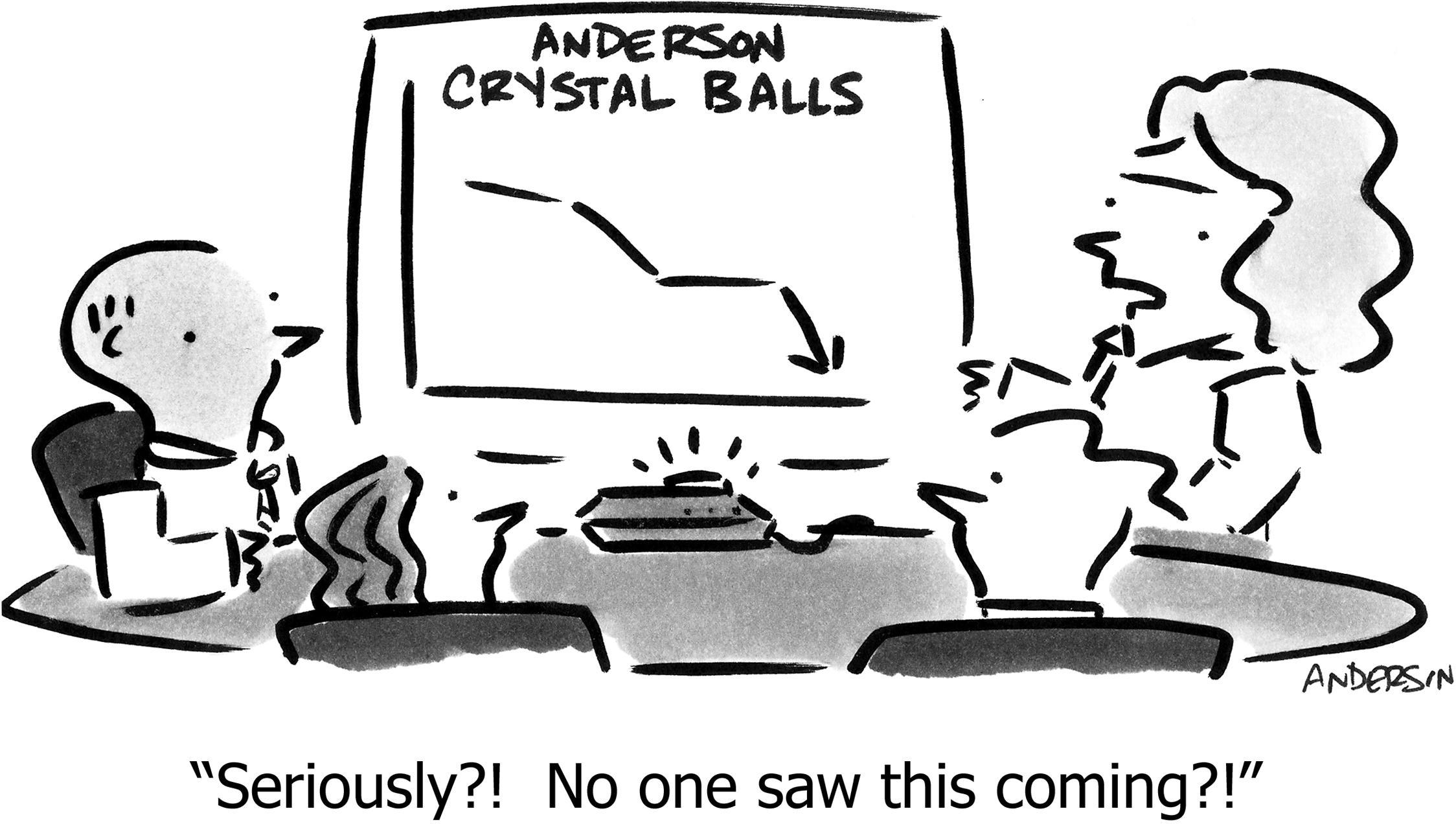
Discernment Error
Consider the life of a forecaster in Antofagasta, Chile, where on average it rains only five days a year (for a grand total of 1.7 millimeters of annual rainfall!). At first glance it seems easy to be a forecaster—just predict “no rain” every day.
Although that forecaster would have low error, she would also be undiscerning. But wait… how could a forecaster ever be discerning in Antofagasta? To be discerning you need to make varied predictions. But reality isn’t varied, so any predictions that were varied, would necessarily be wrong! In a sense, there’s no “space” for discernment, because there’s no variation to discern between. It’s not fair to ask the forecaster to be more discerning than the variation that is actually available to discern.
Compare that with forecaster in Portland, Oregon, USA where it rains 164 days out of the year—about 45%. And there’s no “rainy season”—it’s just chaotic. Here even just predicting 55% or 35% here and there could still be highly accurate but increase discernment. And a world-class forecaster has the space to create a significant amount of discernment.
So it’s not quite fair to ask “How discerning is the forecaster?” Instead we should ask “How discerning is the forecaster, compared with how much discernment is even possible?”
The maximum amount of discernment possible, given the climactic average  , is:2

In general, the closer the climactic average is to 0% or 100%, the less discernment there can be. The maximum possible discernment of 0.25 is available when the climactic average is 50%, i.e. it’s a coin flip.
2 For the mathematically curious: Maximum discernment happens when the forecast is only 100% or 0%, and when it is completely accurate. If there werepredictions, the positive case will happen
times, and the negative case
times. Discernment in the positive bucket is
and in the negative bucket
. The weighted average is
. Factoring out the common
and canceling with
, we’re left with
.
In the 30% example, the maximum possible discernment is %22%3E%3Cg%20data-mml-node=%22math%22%3E%3Cg%20data-mml-node=%22mstyle%22%3E%3Cg%20data-mml-node=%22TeXAtom%22%20data-mjx-texclass=%22ORD%22%3E%3Cg%20data-mml-node=%22mn%22%3E%3Cpath%20data-c=%2230%22%20d=%22M96%20585q56%2081%20153%2081%2048%200%2096-26t78-92q37-83%2037-228%200-155-43-237-20-42-55-67T301-15t-51-7q-26%200-52%206T137%2016%2082%2083Q39%20165%2039%20320q0%20174%2057%20265zm225%2012q-30%2032-71%2032-42%200-72-32-25-26-33-72t-8-192q0-158%208-208t36-79q28-30%2069-30%2040%200%2068%2030%2029%2030%2036%2084t8%20203q0%20145-8%20191t-33%2073z%22/%3E%3Cpath%20data-c=%222E%22%20d=%22M78%2060q0%2024%2017%2042t43%2018q24%200%2042-16t19-43q0-25-17-43T139%200%2096%2017%2078%2060z%22%20transform=%22translate(500,0)%22/%3E%3Cpath%20data-c=%2233%22%20d=%22M127%20463q-27%200-42%2017T69%20524q0%2055%2048%2098t116%2043q35%200%2044-1%2074-12%20113-53t40-89q0-52-34-101t-94-71l-3-2q0-1%209-3t29-9%2038-21q82-53%2082-140%200-79-62-138T238-22q-80%200-138%2043T42%20130q0%2028%2018%2045t45%2018q28%200%2046-18t18-45q0-11-3-20t-7-16-11-12-12-8-10-4-8-3l-4-1q51-45%20124-45%2055%200%2083%2053%2017%2033%2017%20101v20q0%2095-64%20127-15%206-61%207l-42%201-3%202q-2%203-2%2016%200%2018%208%2018%2028%200%2058%205%2034%205%2062%2042t28%20112v8q0%2057-35%2079-22%2014-47%2014-32%200-59-11t-38-23-11-12h3q3-1%208-2t10-5%2012-7%2010-11%208-15%203-20q0-22-14-39t-45-18z%22%20transform=%22translate(778,0)%22/%3E%3Cpath%20data-c=%2230%22%20d=%22M96%20585q56%2081%20153%2081%2048%200%2096-26t78-92q37-83%2037-228%200-155-43-237-20-42-55-67T301-15t-51-7q-26%200-52%206T137%2016%2082%2083Q39%20165%2039%20320q0%20174%2057%20265zm225%2012q-30%2032-71%2032-42%200-72-32-25-26-33-72t-8-192q0-158%208-208t36-79q28-30%2069-30%2040%200%2068%2030%2029%2030%2036%2084t8%20203q0%20145-8%20191t-33%2073z%22%20transform=%22translate(1278,0)%22/%3E%3C/g%3E%3Cg%20data-mml-node=%22mo%22%20transform=%22translate(1778,0)%22%3E%3Cpath%20data-c=%2228%22%20d=%22M94%20250q0%2069%2010%20131t23%20107%2037%2088%2038%2067%2042%2052%2033%2034%2025%2021h13%204q14%200%2014-9%200-3-17-21t-41-53-49-86-42-138-17-193T184%2058%20225-81t49-86%2042-53%2017-21q0-9-15-9h-3-13l-28%2024Q180-141%20137-14T94%20250z%22/%3E%3C/g%3E%3Cg%20data-mml-node=%22mn%22%20transform=%22translate(2167,0)%22%3E%3Cpath%20data-c=%2231%22%20d=%22M213%20578l-13-5q-14-5-40-10t-58-7H83v46h19q47%202%2087%2015t56%2024%2028%2022q2%203%2012%203%209%200%2017-6V361l1-3e2q7-7%2012-9t24-4%2062-2h26V0H416Q395%203%20257%203%20121%203%201e2.0H88V46h26q22%200%2038%200t25%201%2016%203%208%202%206%205%206%204V578z%22/%3E%3C/g%3E%3Cg%20data-mml-node=%22mo%22%20transform=%22translate(2889.2,0)%22%3E%3Cpath%20data-c=%222212%22%20d=%22M84%20237t0%2013%2014%2020H679q15-8%2015-20t-15-20H98q-14%207-14%2020z%22/%3E%3C/g%3E%3Cg%20data-mml-node=%22mn%22%20transform=%22translate(3889.4,0)%22%3E%3Cpath%20data-c=%2230%22%20d=%22M96%20585q56%2081%20153%2081%2048%200%2096-26t78-92q37-83%2037-228%200-155-43-237-20-42-55-67T301-15t-51-7q-26%200-52%206T137%2016%2082%2083Q39%20165%2039%20320q0%20174%2057%20265zm225%2012q-30%2032-71%2032-42%200-72-32-25-26-33-72t-8-192q0-158%208-208t36-79q28-30%2069-30%2040%200%2068%2030%2029%2030%2036%2084t8%20203q0%20145-8%20191t-33%2073z%22/%3E%3Cpath%20data-c=%222E%22%20d=%22M78%2060q0%2024%2017%2042t43%2018q24%200%2042-16t19-43q0-25-17-43T139%200%2096%2017%2078%2060z%22%20transform=%22translate(500,0)%22/%3E%3Cpath%20data-c=%2233%22%20d=%22M127%20463q-27%200-42%2017T69%20524q0%2055%2048%2098t116%2043q35%200%2044-1%2074-12%20113-53t40-89q0-52-34-101t-94-71l-3-2q0-1%209-3t29-9%2038-21q82-53%2082-140%200-79-62-138T238-22q-80%200-138%2043T42%20130q0%2028%2018%2045t45%2018q28%200%2046-18t18-45q0-11-3-20t-7-16-11-12-12-8-10-4-8-3l-4-1q51-45%20124-45%2055%200%2083%2053%2017%2033%2017%20101v20q0%2095-64%20127-15%206-61%207l-42%201-3%202q-2%203-2%2016%200%2018%208%2018%2028%200%2058%205%2034%205%2062%2042t28%20112v8q0%2057-35%2079-22%2014-47%2014-32%200-59-11t-38-23-11-12h3q3-1%208-2t10-5%2012-7%2010-11%208-15%203-20q0-22-14-39t-45-18z%22%20transform=%22translate(778,0)%22/%3E%3Cpath%20data-c=%2230%22%20d=%22M96%20585q56%2081%20153%2081%2048%200%2096-26t78-92q37-83%2037-228%200-155-43-237-20-42-55-67T301-15t-51-7q-26%200-52%206T137%2016%2082%2083Q39%20165%2039%20320q0%20174%2057%20265zm225%2012q-30%2032-71%2032-42%200-72-32-25-26-33-72t-8-192q0-158%208-208t36-79q28-30%2069-30%2040%200%2068%2030%2029%2030%2036%2084t8%20203q0%20145-8%20191t-33%2073z%22%20transform=%22translate(1278,0)%22/%3E%3C/g%3E%3Cg%20data-mml-node=%22mo%22%20transform=%22translate(5667.4,0)%22%3E%3Cpath%20data-c=%2229%22%20d=%22M60%20749l4%201q5%200%2010%200H86l28-24q94-85%20137-212t43-264q0-68-10-131T261%2012%20224-76t-38-67-41-51-32-33-23-19q-3-3-4-4H74q-8%200-11%200t-5%203-3%209q1%201%2011%2013Q221-64%20221%20250T66%20725q-10%2012-11%2013%200%208%205%2011z%22/%3E%3C/g%3E%3Cg%20data-mml-node=%22mo%22%20transform=%22translate(6334.2,0)%22%3E%3Cpath%20data-c=%223D%22%20d=%22M56%20347q0%2013%2014%2020H707q15-8%2015-20%200-11-14-19l-318-1H72q-16%205-16%2020zm0-194q0%2015%2016%2020H708q14-10%2014-20%200-13-15-20H70q-14%207-14%2020z%22/%3E%3C/g%3E%3Cg%20data-mml-node=%22mn%22%20transform=%22translate(7390,0)%22%3E%3Cpath%20data-c=%2230%22%20d=%22M96%20585q56%2081%20153%2081%2048%200%2096-26t78-92q37-83%2037-228%200-155-43-237-20-42-55-67T301-15t-51-7q-26%200-52%206T137%2016%2082%2083Q39%20165%2039%20320q0%20174%2057%20265zm225%2012q-30%2032-71%2032-42%200-72-32-25-26-33-72t-8-192q0-158%208-208t36-79q28-30%2069-30%2040%200%2068%2030%2029%2030%2036%2084t8%20203q0%20145-8%20191t-33%2073z%22/%3E%3Cpath%20data-c=%222E%22%20d=%22M78%2060q0%2024%2017%2042t43%2018q24%200%2042-16t19-43q0-25-17-43T139%200%2096%2017%2078%2060z%22%20transform=%22translate(500,0)%22/%3E%3Cpath%20data-c=%2232%22%20d=%22M109%20429q-27%200-43%2018T50%20491q0%2071%2053%20123t132%2052q91%200%20152-56t62-145q0-43-20-82t-48-68-80-74q-36-31-1e2-92L142%2093l76-1q157%200%20167%205%207%202%2024%2089v3h40v-3q-1-3-13-91T421%203V0H50V19%2031q0%207%206%2015T86%2081q29%2032%2050%2056%209%2010%2034%2037t34%2037%2029%2033%2028%2034%2023%2030%2021%2032%2015%2029%2013%2032%207%2030%203%2033q0%2063-34%20109t-97%2046q-33%200-58-17t-35-33-10-19q0-1%205-1%2018%200%2037-14t19-46q0-25-16-42t-45-18z%22%20transform=%22translate(778,0)%22/%3E%3Cpath%20data-c=%2231%22%20d=%22M213%20578l-13-5q-14-5-40-10t-58-7H83v46h19q47%202%2087%2015t56%2024%2028%2022q2%203%2012%203%209%200%2017-6V361l1-3e2q7-7%2012-9t24-4%2062-2h26V0H416Q395%203%20257%203%20121%203%201e2.0H88V46h26q22%200%2038%200t25%201%2016%203%208%202%206%205%206%204V578z%22%20transform=%22translate(1278,0)%22/%3E%3C/g%3E%3C/g%3E%3C/g%3E%3C/g%3E%3C/g%3E%3C/svg%3E) . Forecaster B’s discernment of 0.04 is therefore not too impressive—plenty of room for improvement. Although still of course B is better than A, who had no discernment whatsoever.
. Forecaster B’s discernment of 0.04 is therefore not too impressive—plenty of room for improvement. Although still of course B is better than A, who had no discernment whatsoever.
In the case of the desert, with a climactic average of %22%3E%3Cg%20data-mml-node=%22math%22%3E%3Cg%20data-mml-node=%22mstyle%22%3E%3Cg%20data-mml-node=%22TeXAtom%22%20data-mjx-texclass=%22ORD%22%3E%3Cg%20data-mml-node=%22mn%22%3E%3Cpath%20data-c=%2235%22%20d=%22M164%20157q0-24-16-40t-39-16h-7q46-79%20122-79%2070%200%20102%2060%2019%2033%2019%20128%200%20103-27%20139-26%2033-58%2033h-6q-78%200-118-68-4-7-7-8t-15-2q-17%200-19%206-2%204-2%20175V614q0%2050%205%2050%202%202%204%202%201%200%2021-8t55-16%2075-8q71%200%20136%2028%208%204%2013%204%208%200%208-18V635q-82-97-205-97-31%200-56%206l-10%202V374q19%2014%2030%2022t36%2016%2051%208q81%200%20137-65t56-154q0-92-64-157T229-22Q148-22%2099%2032T50%20154q0%2024%2011%2038t23%2018%2023%204q25%200%2041-17t16-40z%22/%3E%3C/g%3E%3Cg%20data-mml-node=%22TeXAtom%22%20data-mjx-texclass=%22ORD%22%20transform=%22translate(500,0)%22%3E%3Cg%20data-mml-node=%22mo%22%3E%3Cpath%20data-c=%222F%22%20d=%22M423%20750q9%200%2015-6t6-14q0-5-173-482T92-240q-7-10-17-10-7%200-13%205t-6%2014q0%2010%20174%20488T407%20740q4%2010%2016%2010z%22/%3E%3C/g%3E%3C/g%3E%3Cg%20data-mml-node=%22mn%22%20transform=%22translate(1000,0)%22%3E%3Cpath%20data-c=%2233%22%20d=%22M127%20463q-27%200-42%2017T69%20524q0%2055%2048%2098t116%2043q35%200%2044-1%2074-12%20113-53t40-89q0-52-34-101t-94-71l-3-2q0-1%209-3t29-9%2038-21q82-53%2082-140%200-79-62-138T238-22q-80%200-138%2043T42%20130q0%2028%2018%2045t45%2018q28%200%2046-18t18-45q0-11-3-20t-7-16-11-12-12-8-10-4-8-3l-4-1q51-45%20124-45%2055%200%2083%2053%2017%2033%2017%20101v20q0%2095-64%20127-15%206-61%207l-42%201-3%202q-2%203-2%2016%200%2018%208%2018%2028%200%2058%205%2034%205%2062%2042t28%20112v8q0%2057-35%2079-22%2014-47%2014-32%200-59-11t-38-23-11-12h3q3-1%208-2t10-5%2012-7%2010-11%208-15%203-20q0-22-14-39t-45-18z%22/%3E%3Cpath%20data-c=%2236%22%20d=%22M42%20313q0%20163%2081%20258t180%2095q69%200%2099-36t30-80q0-25-14-40t-39-15q-23%200-38%2014t-15%2039q0%2044%2047%2053-22%2022-62%2025-71%200-117-60-47-66-47-202l1-4q5%206%208%2013%2041%2060%20107%2060h4q46%200%2081-19%2024-14%2048-40t39-57q21-49%2021-107V192q0-23-5-43-11-59-64-115T253-22q-28%200-54%208T143%2016%2092%2075%2056%20172%2042%20313zm215%2084q-30%200-52-17t-34-45-17-57-6-62q0-83%2012-119t38-58q24-18%2053-18%2051%200%2078%2038%2013%2018%2018%2045t5%20105q0%2080-5%20107t-18%2045q-27%2036-72%2036z%22%20transform=%22translate(500,0)%22/%3E%3Cpath%20data-c=%2235%22%20d=%22M164%20157q0-24-16-40t-39-16h-7q46-79%20122-79%2070%200%20102%2060%2019%2033%2019%20128%200%20103-27%20139-26%2033-58%2033h-6q-78%200-118-68-4-7-7-8t-15-2q-17%200-19%206-2%204-2%20175V614q0%2050%205%2050%202%202%204%202%201%200%2021-8t55-16%2075-8q71%200%20136%2028%208%204%2013%204%208%200%208-18V635q-82-97-205-97-31%200-56%206l-10%202V374q19%2014%2030%2022t36%2016%2051%208q81%200%20137-65t56-154q0-92-64-157T229-22Q148-22%2099%2032T50%20154q0%2024%2011%2038t23%2018%2023%204q25%200%2041-17t16-40z%22%20transform=%22translate(1000,0)%22/%3E%3C/g%3E%3Cg%20data-mml-node=%22mo%22%20transform=%22translate(2777.8,0)%22%3E%3Cpath%20data-c=%223D%22%20d=%22M56%20347q0%2013%2014%2020H707q15-8%2015-20%200-11-14-19l-318-1H72q-16%205-16%2020zm0-194q0%2015%2016%2020H708q14-10%2014-20%200-13-15-20H70q-14%207-14%2020z%22/%3E%3C/g%3E%3Cg%20data-mml-node=%22mn%22%20transform=%22translate(3833.6,0)%22%3E%3Cpath%20data-c=%2230%22%20d=%22M96%20585q56%2081%20153%2081%2048%200%2096-26t78-92q37-83%2037-228%200-155-43-237-20-42-55-67T301-15t-51-7q-26%200-52%206T137%2016%2082%2083Q39%20165%2039%20320q0%20174%2057%20265zm225%2012q-30%2032-71%2032-42%200-72-32-25-26-33-72t-8-192q0-158%208-208t36-79q28-30%2069-30%2040%200%2068%2030%2029%2030%2036%2084t8%20203q0%20145-8%20191t-33%2073z%22/%3E%3Cpath%20data-c=%222E%22%20d=%22M78%2060q0%2024%2017%2042t43%2018q24%200%2042-16t19-43q0-25-17-43T139%200%2096%2017%2078%2060z%22%20transform=%22translate(500,0)%22/%3E%3Cpath%20data-c=%2230%22%20d=%22M96%20585q56%2081%20153%2081%2048%200%2096-26t78-92q37-83%2037-228%200-155-43-237-20-42-55-67T301-15t-51-7q-26%200-52%206T137%2016%2082%2083Q39%20165%2039%20320q0%20174%2057%20265zm225%2012q-30%2032-71%2032-42%200-72-32-25-26-33-72t-8-192q0-158%208-208t36-79q28-30%2069-30%2040%200%2068%2030%2029%2030%2036%2084t8%20203q0%20145-8%20191t-33%2073z%22%20transform=%22translate(778,0)%22/%3E%3Cpath%20data-c=%2231%22%20d=%22M213%20578l-13-5q-14-5-40-10t-58-7H83v46h19q47%202%2087%2015t56%2024%2028%2022q2%203%2012%203%209%200%2017-6V361l1-3e2q7-7%2012-9t24-4%2062-2h26V0H416Q395%203%20257%203%20121%203%201e2.0H88V46h26q22%200%2038%200t25%201%2016%203%208%202%206%205%206%204V578z%22%20transform=%22translate(1278,0)%22/%3E%3Cpath%20data-c=%2233%22%20d=%22M127%20463q-27%200-42%2017T69%20524q0%2055%2048%2098t116%2043q35%200%2044-1%2074-12%20113-53t40-89q0-52-34-101t-94-71l-3-2q0-1%209-3t29-9%2038-21q82-53%2082-140%200-79-62-138T238-22q-80%200-138%2043T42%20130q0%2028%2018%2045t45%2018q28%200%2046-18t18-45q0-11-3-20t-7-16-11-12-12-8-10-4-8-3l-4-1q51-45%20124-45%2055%200%2083%2053%2017%2033%2017%20101v20q0%2095-64%20127-15%206-61%207l-42%201-3%202q-2%203-2%2016%200%2018%208%2018%2028%200%2058%205%2034%205%2062%2042t28%20112v8q0%2057-35%2079-22%2014-47%2014-32%200-59-11t-38-23-11-12h3q3-1%208-2t10-5%2012-7%2010-11%208-15%203-20q0-22-14-39t-45-18z%22%20transform=%22translate(1778,0)%22/%3E%3C/g%3E%3Cg%20data-mml-node=%22mi%22%20transform=%22translate(6111.6,0)%22%3E%3Cpath%20data-c=%2225%22%20d=%22M465%20605q-37%200-71%209t-54%2018-21%209q13-33%2013-93%200-90-39-145t-91-56q-57%200-101%2055T56%20548q0%2089%2045%20145t101%2057q39%200%2070-31%2087-77%20192-77%20116%200%20186%2090%2012%2016%2018%2017%202%201%205%201%209%200%2015-7t5-17Q178-47%20170-52q-4-4-10-4-13%200-18%2011-5%209%200%2018%201%203%20221%20331Q469%20462%20525%20546l56%2084q-53-25-116-25zM207%20385q28%200%2056%2042t29%20121q0%2069-25%20116t-67%2048q-7%200-14-3t-19-11-20-30-13-53q-2-20-2-67V527q0-91%2033-124%2018-18%2038-18h4zM5e2%20146q0%2088%2044%20144t103%2057q52%200%2090-55t39-146T737%200%20646-56Q590-56%20545%200T5e2%20146zM651-18q28%200%2056%2042t29%20122q0%2069-25%20116t-67%2047q-7%200-14-3t-19-11-20-30-13-53q-1-12-1-66V124q0-142%2070-142h4z%22/%3E%3C/g%3E%3C/g%3E%3C/g%3E%3C/g%3E%3C/g%3E%3C/svg%3E) , there’s only 0.0128 potential discernment available.
, there’s only 0.0128 potential discernment available.
In any case, this allows us to compute a metric that is comparable to error, but for discernment:
[ Discernment Error ] = [ Maximum Discernment ] − [Discernment]
That is, if you have no discernment, that’s another type of “error”—your forecast is lacking the descriptive power that would come from being maximally discerning. The more discernment you demonstrate, the less of this “discernment error” you exhibit, and the better your forecast is. Just like the less accuracy error you have, the better your forecast is.
Putting it all together: The Forecasting Error Score
It turns out3 you can simply add accuracy error to discernment error, and arrive at a rigorous metric:
3 See “Further Reading” below for the mathematical justification.
[ Forecast Error ] = [Error] + [ Discernment Error ]
Or, writing out each component:
[ Forecast Error ] = [Error] + [ Maximum Discernment ] − [Discernment]
Here’s a way to see why this math works: Every forecaster’s baseline is to guess the climactic average. That will get you a total score of , because you have no accuracy error, but maximum discernment error.
From there, forecasters will try to deviate from the climactic average. The more they put themselves on the line, the less discernment error they rack up, however they also have to be right! The best forecasters outperform the climactic-average (discernment) by more than the accuracy error they introduce. The overall score tells you who is better. Lower is better, since the score is a “total error.”
It is possible to do worse than the climactic average—to make guesses, but be wrong. You know that’s happening when the total error is larger than the baseline .
Indeed, an alternate and equivalent scoring method divides Forecast Error by , to create a metric where 1 means “equal to the baseline,” 0 means “perfect forecast,” and the amount greater or less than 1 indicates proportionally how much better or worse the forecast is from baseline. This has the virtue of the reader not needing to know the value of in order to understand whether a forecaster is better or worse than the baseline, and by how much.
While the total score is useful, the individual components of accuracy error and discernment are also useful because they help you analyze what’s going on:
| Accuracy Error |
Discern | Meaning | Explanation |
|---|---|---|---|
| ↑ | ↓ | Failure | You’re not segmenting the population, and yet you’re still worse than guessing the climactic average. |
| ↓ | ↓ | Useless | You’re only accurate because you’re just guessing the average. |
| ↑ | ↑ | Try Again | You’re making strong predictions, so at least you’re trying, but you’re not guessing correctly. |
| ↓ | ↑ | Ideal | You’re making strong predictions, and you’re correct. |
Now that you know how to measure forecasts, it’s time for you to build some forecasting models. So go try to better understand your customers and prospects, and use this math to know whether iterations of your model are improving.
Further Reading
- Glenn Brier’s original paper proposing this method in 1950, but without this three-component breakdown that was discovered by Allen Murphy in 1973.
- Brier score on Wikipedia: A more formal explanation including the three-component breakdown (which are labelled and explained differently from my exposition, but which are mathematically identical).
- Stein’s Paradox: An estimator that’s always better than the historical average, but in a way that apparently can’t be true.
https://longform.asmartbear.com/forecast/
© 2007-2026 Jason Cohen
 @asmartbear


