 ePub (Kindle)
 Printable PDF
Distributed Logical Time


Time is notoriously difficult to synchronize in distributed systems. Many algorithms require—or have better characteristics when—any number of independent replicas achieve a single global time-ordering. In particular, it is useful to know that if two events are separated by more than a few seconds in real-time, that they will be correctly ordered, despite replicas having unsynchronized physical clocks.
We’re obviously in no danger of arriving at consensus.
—Warren Buffett
However, operating system clocks are undependable and can even move backward. Furthermore, we don’t want to rely on a “master” or central server. Replicas should be able to arbitrarily join or leave a collective without announcement, operate independently, and communicate with each other peer-to-peer, in any pattern.
Common methods to solve the problem either involve custom infrastructure to achieve tight bounds on the behavior of operating system clocks (e.g. Google TrueTime), or some sort of distributed logical clock such as Vector Clocks. The former is unavailable to most of us, especially if we want our code to run in browsers or laptops or non-Google data centers. The latter suffers from unbounded memory requirements and still results in “conflicts” which are resolved arbitrarily or not at all.
Here we present an algorithm and Golang implementation that meets the objectives, with no assumptions about the behavior of operating system clocks, without vector clocks, and without central coordination.
Objectives & Definitions
Definitions
It’s useful to establish a few definitions and conventions before describing how we achieve a solution:
- RT—Real Time—theoretical omniscient “actual time”. Imagine it as arbitrarily-high-precision UTC time exactly synchronized everywhere. This is not a quantity that any replica can compute; it is for algorithmic discussion only.
- PT—Physical Time—the time reported by the operating system. This is the only notion of “time” that a replica can access.
- LT—Logical Time—our synthetic implementation of “time”, with the properties suggested above and precisely defined below.
XT{expression}means “the type of timeXT, applied to the replicas or events in the expression.” For example,PT{ P<Q }means “the Physical Time on the replicaPis less than the Physical Time on replicaQ.”
Requirements & Assumptions
With this terminology, we can define our assumptions and our requirements for LT precisely:
- PT is arbitrary.
It can move backwards, it does not produce unique values, it might update only rarely, it is never synchronized between two replicas, it can be ahead of or behind RT by an arbitrary and variable amount. The only thing we know is that, over a long duration, it generally increases. - LT always increases.
Whenever LT is requested, it will have increased since the previous request (regardless of PT’s behavior). - If B happens after A in real-time, i.e.
RT{ B>A }, but A and B happen on different replicas:- Correctly ordered in LT when sufficiently time-separated in RT.
IfRT{ B-A } > e, whereeis a small, bounded constant, thenLT{ B>A }also. - Arbitrary LT order if close together in RT.
IfRT{ B-A } < e, then there’s best-effort forLT{ B>A }, but it could beLT{ B<A }. eis small and bounded.
emust be small (e.g. 1-2 seconds), and be a constant, not proportional to some state or configuration.eis the time window inside which we accept events that are incorrectly ordered, so we require this window to be small.- “Happened-before” relation is always correctly ordered in LT.
If A happens, then the two replicas communicate, then B happens, then it is always true thatLT{ B>A }, even ifRT{ B-A } < e.
- Correctly ordered in LT when sufficiently time-separated in RT.
- Skewed PT on one replica doesn’t skew the behavior of the collective.
If one replica’s PT differs significantly from RT, it should still participate properly with the collective; for example it shouldn’t automatically “win” due to the late-skewed PT, or be unable to write a change due to early-skewed PT. - LT uses constant memory.
Use a fixed number of bits to represent LT, regardless of factors like the number of replicas. (Unlike Vector Clocks.) - Decentralized, without “join” or “leave” events.
No leaders, no special designations, no central API. Peers can communicate in arbitrary patterns. Peers never need to announce their joining or leaving the collective. There is no list of peers.
It may sound impossible to achieve the goals of LT given that RT is inaccessible, PT lacks all the properties we need, and replicas aren’t synchronized. It’s fun to see that in fact it can be achieved.
LT inside a single replica
It might seem trivial to create LT within a single replica, but even that requires an algorithm. Typically the operating system is used for PT, but PT can move backwards (e.g. with NTP, with leap-seconds, with manual settings), and is non-unique (e.g. asking for the time in rapid succession often yields the same value from the operating system, due to CPUs being faster than the precision of time), and can drift significantly far away from RT (due to various causes as shown in these examples).
PT will generally increase in the long-run, but we have to “smooth over” the bumps where it is stagnant or decreasing. To do that, we store the “last-seen PT” as well as a counter, and use the following algorithm (plus a mutex for concurrent access):
func GetLT() {
	if PT_Current > PT_LastSeen {
		PT_LastSeen = PT_Current
		Counter = 0
	} else {
		Counter = Counter + 1
	}
	return {PT_LastSeen, Counter}
}
LT is ordered first by PT_LastSeen and then by Counter. So, as long as PT increases, we use it, staying hopefully somewhere near RT (more on this later). But, if PT does not increase, the Counter ensures that LT still increases.
In the following simulation from our golang implementation, we can see how LT monotonically increases even when PT doesn’t:

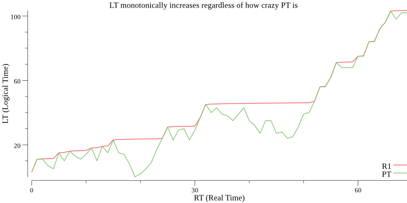
Figure 1
The use of a counter also means the precision of PT is irrelevant. Therefore, a performance optimization is to use a separate recurring timer to update a thread-safe global variable with PT 1-4 times per second, rather than invoking the much more expensive and blocking operating system call to retrieve PT every time we compute LT. With this optimization, we achieved tens of millions of invocations per second even in a Javascript implementation on a typical laptop.
“Happened-Before” relation between replicas
Suppose an event A happens on a replica P, and then P communicates with another replica Q, sending that event. Afterwards, an event B happens on Q. We want to be certain of LT{ B>A }, even though A’s LT was generated on P and B’s LT was generated on Q (Shown in Figure 2).
The PT of P and Q will differ, and could differ in either direction. If PT{ Q>P }, then we’ll get LT{ B>A } naturally, because the PT component of Q is already ahead of the PT component of P. That’s the easy case.
In the other case that PT{ P>Q }, we have a problem. In the example below, P’s PT is one minute ahead of Q’s. After P sends Q event A with LT{ 71.0 }, Q’s LT is still far behind, which means when event B happens one second later, it is LT{ 13.0 }, resulting in the problem LT{ A>B } even though RT{ A<B }:

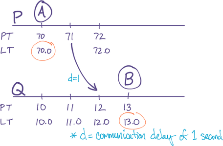
Figure 2: Problem: B’s LT isn’t later than A’s LT, because they’re on different servers.
To fix this, we simply set both components of Q’s LT equal to P’s. Q will know to do this, because when P communicates with Q, it transmits its current value of LT. The following algorithm ensures Q will end up with a strictly-larger LT:
func UpdateLTFromPeer( LT_Peer ) {
	// Operate on current LT
	LT_Local = GetLT()
	// Take the latest LT
	if LT_Peer > LT_Local {
		LT_Local = LT_Peer
	}
	// Ensure strictly larger than any previous LT
	Counter = Counter + 1
	// This is the new local LT
	SaveState(LT_Local)
}
A side effect is that Q’s PT_LastSeen will be ahead of its own PT, but that’s fine because Q will just use its Counter until its own PT catches up. Meanwhile, PT{ B>A } is guaranteed, as the diagram now shows:

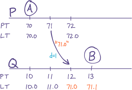
Figure 3: Solution: Q appropriates P’s LT, because LT{ P>Q }
Further discussion and a proof of correctness can be found in the paper that invented this method, in which it is called a Hybrid Logical Clock (HLC).
Using Skew to fix the future
Although the algorithm above satisfies many of the requirements of LT, it violates the requirement that e be small and bounded.
To see why, let’s extend our example to consider what happens with subsequent events on P and Q. In particular, P generates an event C soon after B (in RT), and then Q generates an event D about thirty seconds after that:

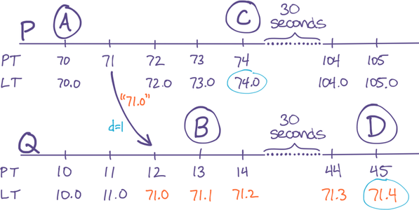
Figure 4: Problem: PT clock-skew breaks LT ordering of future events C and D, even though they differ by 30 seconds in RT
We’ve highlighted the problem: LT{ C>D }, even though RT{ C<D }. The cause of the problem is displayed in the diagram: Because Q’s PT is so far behind P’s, Q has to use its Counter to increment its LT, but meanwhile P is incrementing its LT using its PT. In fact, every event on P during the minute after P communicated with Q will have an LT greater than every event on Q during the same interval, regardless of their ordering in RT. This is the condition described in our original LT goals where events can be mis-ordered in LT if they happen closer than a duration e. The trouble is, e is too big (it’s one minute in this example) and it’s not bounded (it could just as easily be one hour).
This situation remains even after Q’s PT catches up with the synchronization event. P’s LTs will always have a larger PT component than Q’s LTs, and thus P’s events (within any one-minute time window) will always look like they are later than Q’s in LT, regardless of their order in RT.
One solution is to mandate small PT clock skews, which in turn mandates that e is small. For example, a basic NTP service can keep clocks synchronized to within tens of milliseconds. In this case the effect in our example would still exist, but only inside a tiny time window of tens of milliseconds, not a full minute. That would be acceptable.
However, our implementation does not assume control over PT. A replica might be a browser or laptop that we don’t control, or a virtual machine that isn’t running NTP. So, we need an algorithmic extension that eliminates this problem of PT clock skew.
The solution is for Q to compute the PT clock skew, and use that as an offset to its native PT to stay reasonably up-to-date with P. This cannot be done precisely, because of the non-measurable and often-variable communication transmission delay between P and Q, and because PT isn’t dependable, but it turns out being precise is not necessary.
When P communicates its LT to Q, Q computes s = PT{ P-Q } as the “skew.” As the diagram below illustrates, s will always under-estimate the actual clock skew, because it’s not taking transmission-time d into account. In our example here, the actual clock-skew is 60, but the computed skew is 59 due to the transmission delay d=1.
When s is positive, Q saves s. The next time PT is computed, Q uses PT{ Q } + s as physical time. This means Q’s idea of physical time is now only d behind P. This nullifies the problem in our example:

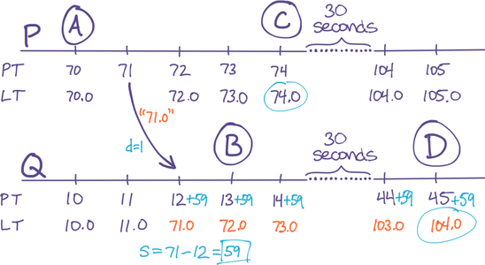
Figure 5: Solution: Use an approximation of real clock skew to reduce the time-window of out-of-order LTs
If s is negative, it is ignored; this ensures that clocks that are already ahead do not get even further ahead.
Although in practice d is not measurable and fluctuates, it is always non-zero, and rarely larger than a few seconds. It is proportional to network transmission time, not proportional to PT clock skew or any other system state or configuration. Therefore we can say that s always under-estimates skew, and by a bounded amount on the order of the replica’s communications delay (i.e. 1ms inside a data center, 100ms across a country, or 1000ms across the world).
Finally, observe from the diagram that the time-window in which this problem can occur has been reduced to just 1 second, i.e. reduced to d. Indeed, e from our LT goals is exactly d theoretically, and on the order of d practically, which we just said was less than a few seconds. Thus, we have achieved the objective that e be a bounded constant.
What happens when all replicas’ PTs are in fact well-synchronized, e.g. with an error less than d, which is easily achievable with well-known algorithms like NTP, or modern phones and laptops that synchronize their clock with GPS? Then the computed skew will be less than zero. To see why, consider that [computed skew] = [real skew] - d, but in this hypothetical, [real skew] might be 50ms whereas d is typically greater than that. Negative computed skews are ignored, thus we’ll always have s = 0.
Although this is not a specific requirement on the behavior of LT, it does satisfy an intuitive desire for skew-correction to vanish when it isn’t needed.
If a replica’s PT is substantially earlier than RT, it will develop a large forward skew, neutralizing the problem. If a replica’s PT is substantially later than RT, all other replicas will develop a skew that aligns with it. Therefore, we achieve the objective that significant skews in either direction don’t adversely affect operation of those replicas or of others.
Still, a replica with a large PT-RT will create a large skew value for the whole group, with the legal but undesirable effect that PT + s differs significantly from RT. When that happens, it’s important that skews don’t continue to creep up, with each replica edging the others forward. A non-zero value of d helps; in our implementation we add another 500ms to the effective value of d to ensure this effect.
Simulations
The following simulations were generated from our Golang implementation.
Convergent LT, with staggered PT
With replicas starting with PT staggered every 10-seconds, one-way-synchronizing a random pair once per second, they monotonically increase and eventually converge on the one with the latest LT:

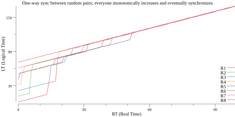
Figure 6
Convergent LT, with variable-rate PT
With each replica’s PT clock running at a different rate relative to RT, one-way-synchronizing a random pair once per second, all replicas keep converging close to the one with the latest LT, i.e. the fastest clock:
Figure 7
Far-Future replica joins, then leaves
A replica with a far-future date joins; all replicas converge on the new far-future LT by one-way-synchronizing a random pair once per second. The “bad” replica then leaves the collective. The remaining replicas have large skews, which should not change. In particular, they should not “creep up” in skew:
Figure 8
Problems
LT at start-up
When a replica first starts up, it will have an LT that is likely to need skew-correction. It should “fix” its LT prior to using it in a meaningful way.
One fix is to communicate with any other replica; this will bring it up to speed and set an appropriate skew.
Another fix is to persist the LT state between runs of the replica. In particular, saving the skew value. However, this is not as good as communicating with a live replica, because the behavior of PT or the collective value of the skew might have changed since the previous run.
Using LT without doing those things is still legal and consistent, but will generate events that will appear to be older than they actually are, relative to other events being generated by other replicas around the same RT.
Anti-Objectives
The following are not goals. In some cases the algorithm gives best-effort to achieve them anyway. In some cases there are things the library user can opt-into having that goal, possibly at the expense of a different goal or constraint.
Uniqueness
The algorithm above creates locally-unique values (i.e. monotonically-increasing), but not globally-unique (i.e. two replicas can generate the same LT).
Uniqueness can be useful because it allows LT to also serve as a “name” of an event in logs or databases.
It’s easy to add uniqueness. Just add more (least-significant) bits to the LT structure. Set them equal to something unique to a replica. This can be a replica ID that is unique in the world, since the rest of the Time components will never be generated again on that replica. Or it can be a sufficiently large number of random bits.
It may seem like collisions are already unlikely, however they are common under certain assumptions, namely if PT is coarsely updated and d is very small. Consider the example above, but rather than d=1, assume a fast network where d=0.001 but a PT source that updates only once per second (on a timer, say). Once P and Q share LT, they will be identical at the same point in RT, and stay synchronized thanks to s. So they will likely collide if both generate an LT inside the same RT second.
Keep PT close to RT
It’s nice if PT stays close to RT, but it is not a requirement.
You can achieve this, in fact making the difference bounded, if you disable skew. This keeps PT close to RT but results in a potentially large e, and thus you get mis-ordered events. If you accept this trade-off, you can ensure PT never strays too far from RT, as proved in the
the HLC paper.
To achieve this while not giving up the objectives on the small size of e, you can use NTP or a similar service to keep PT close to RT.
In the end, the algorithm is simple, and perhaps even obvious in retrospect. The best things are. Simplicity is a core requirement for scalability and truly bug-free code. We hope these properties result in people using this technique.
https://longform.asmartbear.com/distributed-logical-time/
© 2007-2026 Jason Cohen
 @asmartbear


